Getting started tutorial
This introductory tutorial shows how to define a parameter estimation problem in PEtab.jl by constructing a PEtabODEProblem, how to estimate its parameters, and how to assess practical identifiability using profile likelihood analysis.
Input problem
As a running example, we use the Michaelis-Menten enzyme kinetics model:
Using mass-action kinetics, this yields the ODE system:
We assume initial conditions for [S, E, SE, P]:
and that we have measurements of two observables:
We estimate [c1, c2, S0] and assume c3 = 3.0 is known. This tutorial builds the corresponding PEtabODEProblem and estimates these parameters.
Creating a parameter estimation problem
A PEtab parameter estimation problem (PEtabODEProblem) is defined by:
Dynamic model: A Catalyst
ReactionSystemor ModelingToolkitBaseODESystem.Observables:
PEtabObservables that map model states/parameters to measured quantities, including noise models (observable + noise formula).Parameters:
PEtabParameters specifying which parameters are estimated (and optional priors, bounds, and scale).Measurements: Measurement data as a
DataFramein the format described below.Simulation conditions (optional):
PEtabConditions for measurements collected under different experimental conditions, where simulations use different control parameters and/or initial values (see Simulation conditions tutorial).
Defining the dynamic model
The dynamic model can be provided as either a Catalyst ReactionSystem or a ModelingToolkitBase ODESystem. It is recommended to define default parameter values, initial conditions, and (when possible) observables directly in the model system.
For the Michaelis–Menten problem above, the ReactionSystem representation is:
using Catalyst
rn = @reaction_network begin
    @parameters S0 c3=3.0
    @species begin
        S(t) = S0
        E(t) = 50.0
        SE(t) = 0.0
        P(t) = 0.0
    end
    @observables begin
        obs1 ~ S + E
        obs2 ~ P
    end
    c1, S + E --> SE
    c2, SE --> S + E
    c3, SE --> P + E
end
Constant parameters (e.g. c3) and parameters used in initial conditions (e.g. S0) should be declared in @parameters. Parameters that will be estimated (here c1, c2, S0) do not need values in the system. Any species or parameters without specified values default to 0.0.
Using a ODESystem, the model is defined as:
using ModelingToolkitBase
using ModelingToolkitBase: t_nounits as t, D_nounits as D
ps = @parameters S0 c1 c2 c3=3.0
sps = @variables S(t) = S0 E(t) = 50.0 SE(t) = 0.0 P(t) = 0.0 obs1(t) obs2(t)
eqs = [
    # Dynamics
    D(S) ~ -c1 * S * E + c2 * SE
    D(E) ~ -c1 * S * E + c2 * SE + c3 * SE
    D(SE) ~ c1 * S * E - c2 * SE - c3 * SE
    D(P) ~ c3 * SE
    # Observables
    obs1 ~ S + E
    obs2 ~ P
]
@named sys_model = System(eqs, t, sps, ps)
sys = mtkcompile(sys_model)
For an ODESystem, all parameters and states must be declared in the model definition. Any parameter/state left without a value (and not estimated) defaults to 0.0.
Defining observables
To link model outputs to measurements, each measured quantity needs an observable formula and a noise formula. This is specified with PEtabObservable. Since the model system already defines observables (obs1, obs2 above), they can be referenced by name. For example, assume obs1 = S + E is measured with known noise σ = 3.0:
using PEtab
petab_obs1 = PEtabObservable(:petab_obs1, :obs1, 3.0)
PEtabObservable petab_obs1: data ~ Normal(μ=obs1, σ=3.0)The first argument is the observable_id used to link measurement rows in the measurement table (see below) to this PEtabObservable. The second argument (:obs1) references the observable defined in the model system, and the third is the noise parameter. By default, measurements are assumed Normally distributed (other distributions can be selected via the distribution keyword).
The noise level can also be estimated. Assume we measure obs2 = P with unknown noise parameter sigma:
@parameters sigma
petab_obs2 = PEtabObservable(:petab_obs2, :obs2, sigma)
PEtabObservable petab_obs2: data ~ Normal(μ=obs2, σ=sigma)Finally, all observables should be collected into a Vector:
observables = [petab_obs1, petab_obs2]Defining parameters to estimate
Parameters to estimate are specified with PEtabParameter. For example, to estimate c1:
p_c1 = PEtabParameter(:c1)PEtabParameter c1: estimate (scale = log10, bounds = [1.0e-03, 1.0e+03])By default, parameters are assigned bounds [1e-3, 1e3] and estimated on a log10 scale (can be changed via keyword arguments). These defaults typically improve parameter estimation performance performance [2–4]), Parameters can also be assigned priors. For example, to assign a LogNormal(1.0, 0.3) prior to c2:
using Distributions
p_c2 = PEtabParameter(:c2; prior = LogNormal(1.0, 0.3))
PEtabParameter c2: estimate (scale = log10, prior(c2) = LogNormal(μ=1.0, σ=0.3))All parameters to estimate should be defined similarly, and collected into a Vector:
p_S0 = PEtabParameter(:S0)
p_sigma = PEtabParameter(:sigma)
pest = [p_c1, p_c2, p_S0, p_sigma]
4-element Vector{PEtabParameter}:
PEtabParameter c1: estimate (scale = log10, bounds = [1.0e-03, 1.0e+03])
PEtabParameter c2: estimate (scale = log10, prior(c2) = LogNormal(μ=1.0, σ=0.3))
PEtabParameter S0: estimate (scale = log10, bounds = [1.0e-03, 1.0e+03])
PEtabParameter sigma: estimate (scale = log10, bounds = [1.0e-03, 1.0e+03])Measurement data format
Measurement data is provided as a DataFrame with the following columns (order does not matter):
| obs_id (str) | time (float) | measurement (float) |
|---|---|---|
| id | val | val |
| ... | ... | ... |
obs_id: Observable id identifying whichPEtabObservablethe row belongs to.time: Measurement time point.measurement: Measured value.
For our working example, using simulated data, a valid measurement table could be:
using OrdinaryDiffEqRosenbrock, DataFrames
# Simulate with 'true' parameters
ps = [:c1 => 1.0, :c2 => 10.0, :c3 => 3.0, :S0 => 100.0]
u0 = [:E => 50.0, :SE => 0.0, :P => 0.0]
tspan = (0.0, 10.0)
oprob = ODEProblem(rn, u0, tspan, ps)
sol = solve(oprob, Rodas5P(); saveat = 0:0.5:10.0)

obs1 = (sol[:S] + sol[:E]) .+ randn(length(sol[:E]))
obs2   = sol[:P] .+ randn(length(sol[:P]))

df1 = DataFrame(obs_id = "petab_obs1", time = sol.t, measurement = obs1)
df2   = DataFrame(obs_id = "petab_obs2", time = sol.t, measurement = obs2)
measurements = vcat(df1, df2)| Row | obs_id | time | measurement |
|---|---|---|---|
| String | Float64 | Float64 | |
| 1 | petab_obs1 | 0.0 | 150.637 |
| 2 | petab_obs1 | 0.5 | 36.7498 |
| 3 | petab_obs1 | 1.0 | 40.2087 |
| 4 | petab_obs1 | 1.5 | 46.5594 |
| 5 | petab_obs1 | 2.0 | 50.9807 |
Note that the measurement table follows a tidy/long format [5], where each row is one measurement. For repeats at the same time point, add one row per replicate.
Bringing it all together
Given a model, observables, parameters to estimate, and measurement data, we can build a PEtabODEProblem for parameter estimation. This is a two-step process: first create a PEtabModel, then a PEtabODEProblem.
Regardless of whether the model is a ReactionSystem or an ODESystem, a PEtabModel is created with:
model_rn = PEtabModel(rn, observables, measurements, pest)
model_sys = PEtabModel(sys, observables, measurements, pest)
From a PEtabModel, a PEtabODEProblem is created as:
petab_prob = PEtabODEProblem(model_rn)PEtabODEProblem ReactionSystemModel: 4 parameters to estimate
(for more statistics, call `describe(petab_prob)`)For which a printed summary is obtainable with:
describe(petab_prob)PEtabODEProblem ReactionSystemModel
Problem statistics
Parameters to estimate: 4
ODE: 4 states, 4 parameters
Observables: 2
Simulation conditions: 1
Configuration
Gradient method: ForwardDiff
Hessian method: ForwardDiff
ODE solver (nllh): Rodas5P (abstol=1.0e-08, reltol=1.0e-08, maxiters=1e+04)
ODE solver (grad): Rodas5P (abstol=1.0e-08, reltol=1.0e-08, maxiters=1e+04)The printed summary shows information such as the number of parameters to estimate, the default ODE solver, and default gradients/Hessians computation methods computed. These defaults are tuned for typical biological models (see the Defaults page) and can be customized when constructing PEtabODEProblem.
Next, we estimate the unknown parameters given a PEtabODEProblem.
Parameter estimation
A PEtabODEProblem contains everything needed to run parameter estimation with a numerical optimizer. For convenience, PEtab.jl provides built-in wrappers for several optimizers, including Optim.jl, Ipopt, Optimization.jl, and Fides.jl. This section shows how to estimate parameters with Fides.jl from a starting guess x0, and how to use multistart optimization to mitigate local minima.
Single-start parameter estimation
Numerical optimizers require a starting point x0 in the parameter order expected by the PEtabODEProblem. A simple option is to use the nominal values from PEtabParameter via get_x:
x0 = get_x(petab_prob)ComponentVector{Float64}(log10_c1 = 2.6989704386302837, log10_c2 = 0.0, log10_S0 = 2.6989704386302837, log10_sigma = 2.6989704386302837)x0 is a ComponentVector, so parameters can be accessed by name. Parameters estimated on a log scale have a prefix such as log10_, and values must be set on that scale, e.g. to set c1 = 10.0:
x0.log10_c1 = log10(10.0)To reduce bias in parameter estimation, it is often best to randomly sample x0 within the parameter bounds:
x0 = get_startguesses(petab_prob, 1)Given x0, we can estimate parameters. For this small example (4 parameters), we use the Newton-trust region method from Fides.jl with the Hessian computed by petab_prob (CustomHessian):
using Fides
res = calibrate(petab_prob, x0, Fides.CustomHessian())
PEtabOptimisationResult
min(f) = 7.21e+01
Parameters estimated = 4
Optimiser iterations = 32
Runtime = 3.3e+00s
Optimiser algorithm = FidesThe printout shows parameter estimation statistics, such as the final objective value fmin (which, since PEtab works with likelihoods, corresponds to the negative log-likelihood). The estimated parameters are available as:
res.xminComponentVector{Float64}(log10_c1 = -0.3943665233456284, log10_c2 = 0.44288231281851825, log10_S0 = 2.0008656741206052, log10_sigma = -0.037263209239521734)Lastly, to evaluate the parameter estimation, it is useful to plot how well the model fits the data:
using Plots
plot(res, petab_prob; linewidth = 2.0)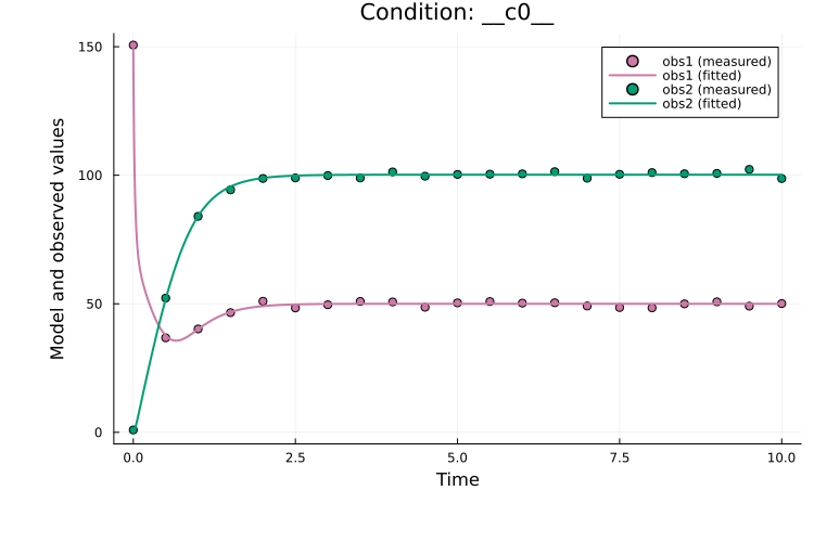
ODE parameter estimation problems often have multiple local minima [3], so a single start may not find the best solution. Next, we cover how to mitigate this with multistart optimization.
Multi-start parameter estimation
In multi-start estimation, the optimizer is run from multiple random starting points to reduce the risk of converging to a local minimum. This simple global optimization strategy has proved effective for ODE models [1, 3, 6].
PEtab.jl provides calibrate_multistart, which generates starting points (by default using Latin hypercube sampling within bounds) and runs the optimizer. For example, to run n = 50 starts with Fides (here using a BFGS Hessian approximation):
using Fides, StableRNGs
rng = StableRNG(42)
ms_res = calibrate_multistart(rng, petab_prob, Fides.BFGS(), 50)
PEtabMultistartResult
min(f) = 7.21e+01
Parameters estimated = 4
Number of multistarts = 50
Optimiser algorithm = FidesPassing an rng ensures reproducible starting points. The printed summary reports the best objective value fmin across runs. A useful diagnostic is the waterfall plot, which shows the final objective value for each start (sorted best to worst):
plot(ms_res; plot_type = :waterfall)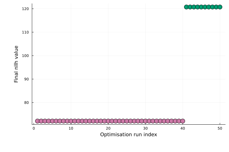
The plateaus correspond to different local optima; the lowest plateau indicates the best solution found across multiple runs. Finally, the best-fit simulation against the data can be plotted as:
plot(ms_res, petab_prob; linewidth = 2.0)
Parallelize multi-start runs
calibrate_multistart can often be sped up by running starts in parallel via the nprocs keyword (see this tutorial).
Identifiability analysis (profile likelihood)
After estimating the parameters, it is useful to assess how precisely they can be determined from the available data, that is, their practical identifiability. Poor identifiability means that multiple parameter values fit the data nearly equally well, making predictions outside the measured conditions unreliable.
A standard approach for this is profile likelihood analysis [7]. A fitted PEtab model can be converted directly to a ProfileLikelihoodProblem:
using LikelihoodProfiler
# First argument can be parameter estimation results
pl_prob = ProfileLikelihoodProblem(ms_res, petab_prob)
# Alternatively, the first argument can be a parameter vector
pl_prob = ProfileLikelihoodProblem(ms_res.xmin, petab_prob)
Given the ProfileLikelihoodProblem, we can compute the profiles as follows:
using OptimizationLBFGSB
meth_opt = OptimizationProfiler(
    optimizer = OptimizationLBFGSB.LBFGSB(),
    stepper = FixedStep(; initial_step = 5e-3)
)
pl_sol = LikelihoodProfiler.solve(pl_prob, meth_opt)
Profile Likelihood solution. Use `sol[i]` to index the computed profiles.Plotting the profiles shows that the model is practically identifiable in this case, as all parameters have finite and well-constrained profiles:
plot(pl_sol)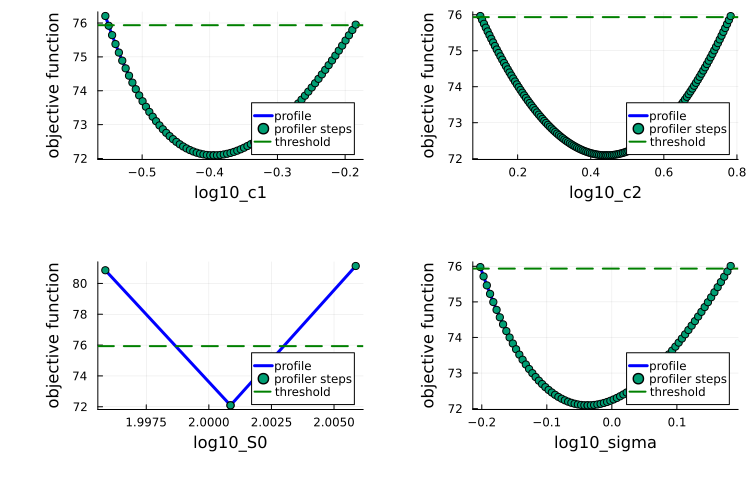
The solution pl_sol supports symbolic indexing. For example, the profile for parameter c1 can be inspected with:
profile_log10_c1 = pl_sol[:log10_c1]
plot(profile_log10_c1)
title!("log10_c1 profile")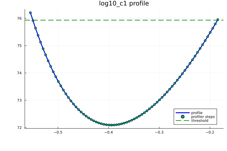
The corresponding confidence interval can then be inspected from the parameter-specific profile solution:
profile_log10_c1Profile curve. Use `plot` to visualize the profile or `DataFrame` to get tabular representation.
Estimated confidence interval (CI): (left = -0.549637827398212, right = -0.18491268296033694)
CI endpoints retcodes: (left = :Identifiable, right = :Identifiable)For more details on available profiling options, see the LikelihoodProfiler.jl documentation. Note that the profile confidence intervals are returned on the parameter estimation scale, which in this example is log10. Transforming the confidence intervals to the linear scale is as simple as applying exp10 to the interval bounds, for example:
ci_log10 = endpoints(profile_log10_c1)
ci = (left = exp10(ci_log10.left), right = exp10(ci_log10.right))
(left = 0.2820734254744012, right = 0.653261880956154)Next steps
This tutorial introduced how to define a PEtabODEProblem. For all available options when building a problem (e.g. options for PEtabParameter), see the API. For additional supported features when setting up a parameter-estimation problem, see the following tutorials:
Simulation conditions: Measurements collected under different experimental conditions (e.g. simulations use different initial values).
Pre-equilibration: Enforce a steady state before the model is matched against data (pre-equilibration).
Simulation condition-specific parameters: Subset of model parameters which are estimated take different across simulation conditions.
Observable and noise parameters: Observable/noise parameters in
PEtabObservableformulas that are not part of the model system (e.g. scale/offset), optionally time-point-specific.Events/callbacks: Time- or state-triggered events/callbacks.
Import PEtab standard format: Load problems from PEtab standard format.
Supported model systems: Supported ways to define the dynamic model (
ReactionSystem,ODESystem, orODEProblem) and available options.
On the top of the functionality for mechanistic models, scientific machine learning (SciML) problems combining machine learning (ML) and mechanistic modules are also supported. For details see:
SciML starter tutorial: Introductory tutorial on how to create and train a SciML problem that combines mechanistic ODE and ML (neural network) models.
Extended UDE tutorial: Define the UDE model as an
ODEProblemfor more control over the problem setup.ML models in observables: define an ML model in the observable formula of a
PEtabObservable(e.g. to correct model misspecification).Pre-simulation ML models: define ML models that map input data (e.g. high-dimensional images) to ODE parameters or initial conditions prior to model simulation.
Importing PEtab SciML: import problems in the PEtab-SciML standard format.
Training strategies: How to improve SciML training (parameter estimation) performance using strategies such as curriculum learning and multiple shooting via PEtabTraining.jl.
In addition to defining a parameter estimation problem, this tutorial showed how to fit parameters using Fides.jl. For more on parameter estimation, see:
Parameter estimation extended tutorial: Extended tutorial on estimation functionality (e.g. multi-start, Optimization.jl integration).
Available optimization algorithms: Supported algorithms and recommended defaults.
Plotting parameter estimation results: Plotting options for parameter estimation output.
Bayesian inference: Sampling-based inference (e.g. NUTS and AdaptiveMCMC).
Identifiability analysis: For more details, see the LikelihoodProfiler.jl documentation and [3, 7].
Lastly, PEtabODEProblem has many configurable options. Defaults are based on extensive benchmarks (see Default PEtabODEProblem options) [1], and available gradient/Hessian settings are summarized in Derivative methods. While these defaults are often performant, they are not optimal for every problem. See the Configuration section for performance tips and tuning guidelines.
Copy pasteable example
using Catalyst, ModelingToolkitBase, PEtab
using ModelingToolkitBase: t_nounits as t, D_nounits as D

rn = @reaction_network begin
    @parameters S0 c3=3.0
    @species begin
        S(t) = S0
        E(t) = 50.0
        SE(t) = 0.0
        P(t) = 0.0
    end
    @observables begin
        obs1 ~ S + E
        obs2 ~ P
    end
    c1, S + E --> SE
    c2, SE --> S + E
    c3, SE --> P + E
end

ps = @parameters S0 c1 c2 c3=3.0
sps = @variables S(t) = S0 E(t) = 50.0 SE(t) = 0.0 P(t) = 0.0 obs1(t) obs2(t)
eqs = [
    # Dynamics
    D(S) ~ -c1 * S * E + c2 * SE
    D(E) ~ -c1 * S * E + c2 * SE + c3 * SE
    D(SE) ~ c1 * S * E - c2 * SE - c3 * SE
    D(P) ~ c3 * SE
    # Observables
    obs1 ~ S + E
    obs2 ~ P
]
@named sys_model = System(eqs, t, sps, ps)
sys = mtkcompile(sys_model)

# Observables
@parameters sigma
petab_obs1 = PEtabObservable(:petab_obs1, :obs1, 3.0)
petab_obs2 = PEtabObservable(:petab_obs2, :obs2, sigma)
observables = [petab_obs1, petab_obs2]

# Parameters to estimate
using Distributions
p_c1 = PEtabParameter(:c1)
p_c2 = PEtabParameter(:c2; prior = LogNormal(2.5, 0.3))
p_S0 = PEtabParameter(:S0)
p_sigma = PEtabParameter(:sigma)
pest = [p_c1, p_c2, p_S0, p_sigma]

# Measurements; simulate with 'true' parameters
using OrdinaryDiffEqRosenbrock, DataFrames
ps = [:c1 => 1.0, :c2 => 10.0, :c3 => 1.0, :S0 => 100.0]
u0 = [:E => 50.0, :SE => 0.0, :P => 0.0]
tspan = (0.0, 10.0)
oprob = ODEProblem(rn, u0, tspan, ps)
sol = solve(oprob, Rodas5P(); saveat = 0:0.5:10.0)
obs1 = (sol[:S] + sol[:E]) .+ randn(length(sol[:E]))
obs2   = sol[:P] .+ randn(length(sol[:P]))
df1 = DataFrame(obs_id = "petab_obs1", time = sol.t, measurement = obs1)
df2   = DataFrame(obs_id = "petab_obs2", time = sol.t, measurement = obs2)
measurements = vcat(df1, df2)

# Create the PEtabODEProblem
model_rn = PEtabModel(rn, observables, measurements, pest)
model_sys = PEtabModel(sys, observables, measurements, pest)
petab_prob = PEtabODEProblem(model_rn)

# Parameter estimation, single start
using Fides, Plots
x0 = get_startguesses(petab_prob, 1)
res = calibrate(petab_prob, x0, Fides.CustomHessian())
plot(res, petab_prob; linewidth = 2.0)

# Multistart parameter estimation
using StableRNGs
rng = StableRNG(42)
ms_res = calibrate_multistart(rng, petab_prob, Fides.BFGS(), 50)
plot(ms_res; plot_type = :waterfall)
plot(ms_res, petab_prob; linewidth = 2.0)

# Profile likelihood analysis
using ComponentArrays, LikelihoodProfiler, OptimizationLBFGSB
pl_prob = ProfileLikelihoodProblem(ms_res, petab_prob)
meth_opt = OptimizationProfiler(
    optimizer = OptimizationLBFGSB.LBFGSB(),
    stepper = FixedStep(; initial_step = 5e-3)
)
pl_sol = LikelihoodProfiler.solve(pl_prob, meth_opt)
xl = permutedims(labels(ms_res.xmin))
p = plot(pl_sol; xlabel = xl)
WARNING: using Fides.solve in module Main conflicts with an existing identifier.
2026-06-25 08:43:39 fides(WARNING) Stopping as maximum number of iterations 1000 was exceeded.References
S. Persson, F. Fröhlich, S. Grein, T. Loman, D. Ognissanti, V. Hasselgren, J. Hasenauer and M. Cvijovic. PEtab. jl: advancing the efficiency and utility of dynamic modelling. Bioinformatics 41, btaf497 (2025).
F. Fröhlich and P. K. Sorger. Fides: Reliable trust-region optimization for parameter estimation of ordinary differential equation models. PLoS computational biology 18, e1010322 (2022).
A. Raue, M. Schilling, J. Bachmann, A. Matteson, M. Schelke, D. Kaschek, S. Hug, C. Kreutz, B. D. Harms, F. J. Theis and others. Lessons learned from quantitative dynamical modeling in systems biology. PloS one 8, e74335 (2013).
H. Hass, C. Loos, E. Raimundez-Alvarez, J. Timmer, J. Hasenauer and C. Kreutz. Benchmark problems for dynamic modeling of intracellular processes. Bioinformatics 35, 3073–3082 (2019).
H. Wickham. Tidy data. Journal of statistical software 59, 1–23 (2014).
A. F. Villaverde, F. Fröhlich, D. Weindl, J. Hasenauer and J. R. Banga. Benchmarking optimization methods for parameter estimation in large kinetic models. Bioinformatics 35, 830–838 (2019).
A. Raue, C. Kreutz, T. Maiwald, J. Bachmann, M. Schilling, U. Klingmüller and J. Timmer. Structural and practical identifiability analysis of partially observed dynamical models by exploiting the profile likelihood. Bioinformatics 25, 1923–1929 (2009).