Tutorial

This tutorial demonstrates how to import an SBML model with SBMLImporter and simulate it as a JumpProblem (Gillespie/SSA), SDEProblem (chemical Langevin), or ODEProblem (deterministic ODEs). It also describes how to modify parameters and initial conditions, as we as how to index solution trajectories by SBML IDs.

Input: a valid SBML file

SBMLImporter only requires one input: a valid SBML file. SBML files can be created from various sources, such as the graphical interface of COPASI, by converting rule-based BioNetGen models, or by using any other SBML exporting tools. Additionally, a large collection of published SBML models are hosted on BioModels.

This tutorial will use the Brusselator model, whose SBML file can be downloaded from this link.

Importing a model

SBML models are imported with load_SBML:

using SBMLImporter
prn, cb = load_SBML(path_sbml; massaction=true)

The keyword massaction=true indicates that reactions follow chemical mass-action kinetics. This enables efficient jump (SSA-type) simulation.

load_SBML returns two outputs: a ParsedReactionSystem (prn) and a CallbackSet (cb). The CallbackSet holds any SBML events, as well as any piecewise functions parsed into events. The ParsedReactionSystem includes a Catalyst ReactionSystem (prn.rn), a map for the initial values of each species (prn.u0), and a map for setting the model parameter values (prn.p). Many modeling tasks can be performed with a Catalyst ReactionSystem. For example, model reactions can be inspected with:

using Catalyst
reactions(prn.rn)

$$\begin{array}{rl}\varnothing & \underset{C}{\overset{AC}{\rightleftharpoons }}\mathrm{X}\\ \mathrm{Y}+2\mathrm{X}& \stackrel{2C}{\to }3\mathrm{X}\\ \mathrm{X}& \stackrel{BC}{\to }\mathrm{Y}\end{array}$$

INFO

The massaction keyword only affects jump simulations. For SDEProblem and ODEProblem workflows, it can be ignored.

Jump simulations

Jump simulations (e.g. Gillespie/SSA) are run by constructing a JumpProblem. This requires an intermediate DiscreteProblem:

using JumpProcesses
tspan = (0.0, 10.0)
dprob = DiscreteProblem(prn.rn, prn.u0, tspan, prn.p)
jprob = JumpProblem(prn.rn, dprob, Direct())

The resulting JumpProblem can be simulated with solvers from JumpProcesses.jl, for example SSAStepper:

using Plots
sol = solve(jprob, SSAStepper(), callback=cb)
plot(sol; xlabel="Time [s]", ylabel="Species amount")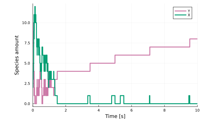

Further details are available in the JumpProcesses.jl documentation. A guide to choosing a jump simulation algorithm can be found here.

SDE simulations

Chemical Langevin simulations are run by constructing an SDEProblem from the reaction system:

using StochasticDiffEq
tspan = (0.0, 10.0)
sprob = SDEProblem(prn.rn, prn.u0, tspan, prn.p)

The SDEProblem can be simulated with solvers from StochasticDiffEq.jl, for example LambaEM:

sol = solve(sprob, LambaEM(), callback=cb)
plot(sol; xlabel="Time [s]", ylabel="Species amount")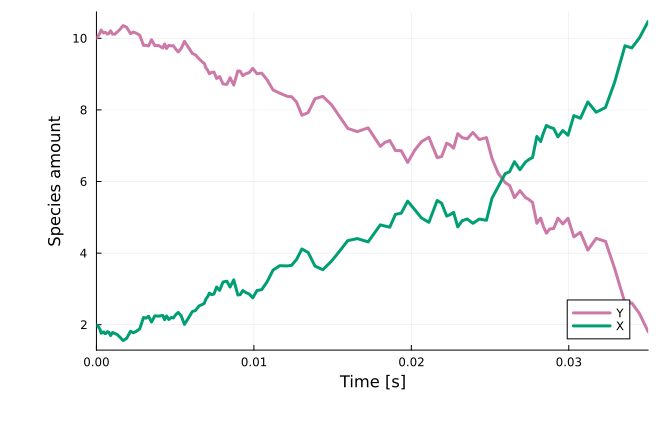

For more information, see the StochasticDiffEq.jl documentation.

ODE simulations

Deterministic simulations can be obtained by converting the reaction system into an ODESystem:

using ModelingToolkit
sys = structural_simplify(convert(ODESystem, prn.rn))

Calling structural_simplify inlines assignment rules into the final equations. As a sanity check, the generated ODEs can be inspected:

equations(sys)

$$\begin{array}{rl}\frac{\mathrm{d}X\left(t\right)}{\mathrm{d}t}& =AC-CX\left(t\right)-BCX\left(t\right)+{\left(X\left(t\right)\right)}^{2}CY\left(t\right)\\ \frac{\mathrm{d}Y\left(t\right)}{\mathrm{d}t}& =BCX\left(t\right)-{\left(X\left(t\right)\right)}^{2}CY\left(t\right)\end{array}$$

An ODEProblem can then be constructed:

using OrdinaryDiffEq
tspan = (0.0, 10.0)
oprob = ODEProblem(sys, prn.u0, tspan, prn.p, jac=true)

With jac=true, the Jacobian is generated symbolically, which often improves performance. The ODEProblem can be simulated with solvers from OrdinaryDiffEq.jl, for example Rodas5P:

sol = solve(oprob, Rodas5P(), callback=cb)
plot(sol; xlabel="Time [s]", ylabel="Species amount")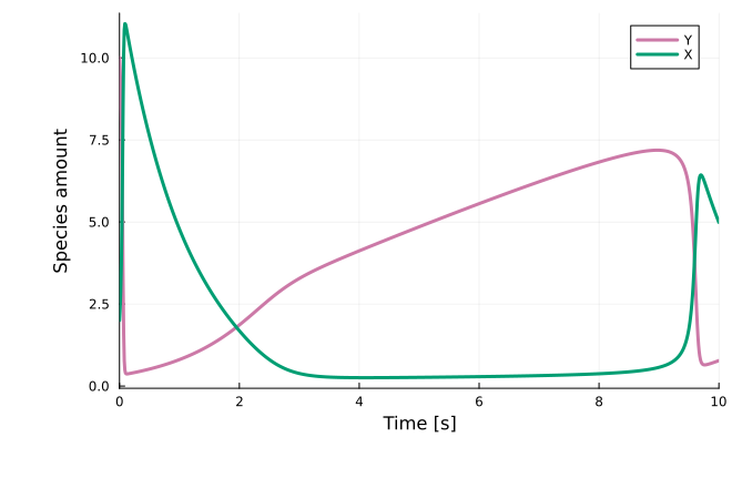

For more information, see the OrdinaryDiffEq.jl documentation. An ODE solver selection guide is available here.

Importing large models

For large models (>1000 species), symbolic Jacobian construction can be time-consuming. If import time dominates, setting jac=false can help.

Indexing parameters, species, and solutions

Problems imported by load_SBML (ODEProblem, SDEProblem, or JumpProblem) support SymbolicIndexingInterface, enabling model variables to be read and updated by SBML IDs.

Parameter values can be modified via prob.ps. For example, parameter A can be set with:

oprob.ps[:A] = 2.0

Initial conditions can be modified by indexing the problem. For example, the initial value of X can be set with:

oprob[:X] = 2.0

After solving, the same symbolic indexing can be used to retrieve trajectories, e.g. for species X:

sol = solve(oprob, Rodas5P(), callback=cb)
sol[:X]

47-element Vector{Float64}:
  2.0
  3.787570124204133
  5.516673430853301
  8.095067081821892
  9.499430337266551
 10.449730413343438
 10.927931715773335
 11.131387019936838
 11.13632911655387
 11.011995418201625
  ⋮
  2.0223722399676944
  2.102868142239643
  2.0600463095856725
  1.981895908508778
  1.9604665946886284
  1.99665547385971
  2.0190286919500253
  1.9995696819688251
  1.991785525596843

The same solution indexing applies to other SBML variables (e.g. assignment rules). If inline_assignment_rules=true was passed to load_SBML, assignment rules are inlined into the model equations during import and cannot be accessed this way.

Next steps

For downstream modeling tasks supported by Catalyst ReactionSystems (e.g. bifurcation analysis), see the Catalyst documentation. For parameter estimation of SBML models, see the PEtab.jl documentation

If importing an SBML model fails, please consult the FAQ first. Additional import options and keyword arguments are documented in the API.