Plotting fitted neural network functions

In addition to the plotting functionality shared for all PEtab problems (see Plotting parameter estimation results), PEtab.jl provides two plot types for inspecting fitted neural network functions in UDE problems:

• Best-fit function: plots the single best-fit neural network function discovered from the data.

• Function ensemble: plots the ensemble of fitted functions across multistart runs, which serves as a measure of functional identifiability.

INFO

Fitted-function plots are currently supported only for models defined as a Catalyst ReactionSystem or ModelingToolkitBase ODESystem, and only for functions with a single input argument (e.g., one Vector) to the neural network.

Plotting the best-fit function

The following UDE examples use a mutual activation loop model fitted to synthetic data. In the model, $X$ and $Y$ activate each other, where the effect of $Y$ on $X$'s production follows a Hill function. We assume this activation function is unknown and attempt to recover it using a UDE. The code below declares the model, generates synthetic data, and fits it. The resulting fitting problem (petab_prob) and calibration result (petab_sol) are used throughout.

# Create model (a mutual activation loop).
using Catalyst
rn = @reaction_network begin
    hill(Y,v,K,n), 0 --> X
    X, 0 --> Y
    d, (X,Y) --> 0
end

# Generate synthetic data.
using Distributions, OrdinaryDiffEqTsit5, Plots
t_measurement = 0.0:1:50.0
u0 = [:X => 2.0, :Y => 0.1]
ps_true = [:v => 1.1, :K => 2.0, :n => 3.0, :d => 0.5]
oprob_true = ODEProblem(rn, u0, t_measurement[end], ps_true)
sol_true = solve(oprob_true, Tsit5())
σ = 0.2
X_true = sol_true(t_measurement; idxs = :X)
X_observed = [rand(Normal(X, σ)) for X in X_true]
Y_true = sol_true(t_measurement; idxs = :Y)
Y_observed = [rand(Normal(Y, σ)) for Y in Y_true]

# Create the UDE.
using ModelingToolkitNeuralNets, Lux
nn_arch = Lux.Chain(
    Lux.Dense(1 => 3, Lux.softplus, use_bias = false),
    Lux.Dense(3 => 3, Lux.softplus, use_bias = false),
    Lux.Dense(3 => 1, Lux.softplus, use_bias = false)
)
@SymbolicNeuralNetwork U, theta = nn_arch
A(x) = U(x, theta)[1]
rn_ude = @reaction_network begin
    $A(Y), 0 --> X
    X, 0 --> Y
    d, (X,Y) --> 0
end

# Create the PEtab problem.
using DataFrames, Optim, PEtab
observables = [
    PEtabObservable(:obs_X, :X, σ),
    PEtabObservable(:obs_Y, :Y, σ)
]
pest = [
    PEtabMLParameter(:theta),
    PEtabParameter(:d; scale = :log10)
]
mX = DataFrame(
    obs_id = "obs_X", time = t_measurement,
    measurement = X_observed
)
mY = DataFrame(
    obs_id = "obs_Y", time = t_measurement,
    measurement = Y_observed
  )
petab_model = PEtabModel(
    rn_ude, observables, vcat(mX, mY), pest; speciemap = u0
)
petab_prob = PEtabODEProblem(petab_model)

# Fit the UDE. Here we load a pre-calibrated result
# It can also be computed via `calibrate_multistart`.
petab_sol = PEtabMultistartResult(path_res)

To plot the best-fit learned function, pass the calibration result and fitting problem to plot with plot_type = :best_function:

plot(petab_sol, petab_prob; plot_type = :best_function)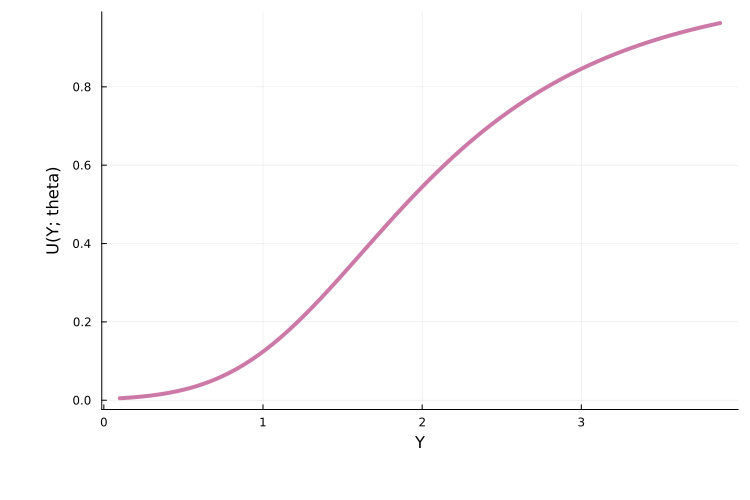

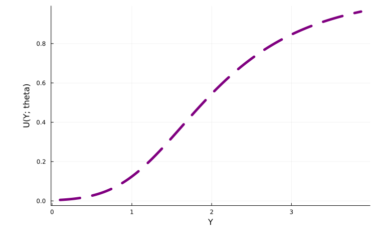
For a multistart run, this plots the function learned by the neural network in the best-performing sub-run. Standard plot attributes can also be passed as keyword arguments:

plot(
    petab_sol, petab_prob; plot_type = :best_function, lw = 5,
    color = :purple, linestyle = :dash
)

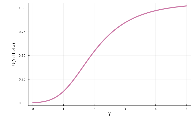
By default, PEtab infers the support of the fitted function from the solution and evaluates it over that range. To set a custom range, or to extrapolate beyond the data support, use the x_support argument:

plot(
    petab_sol, petab_prob; plot_type = :best_function,
    x_support = (0.0, 5.0)
)

Additional options specific to :best_function, with their default values:

• plt_dens = 200: number of evenly spaced grid points over x_support at which the function is evaluated.

• nn_idx = 1: for models with multiple neural networks, selects which network to plot.

• plotted_dim = 1: for functions with multiple output dimensions, selects which dimension to plot.

Plotting the function ensemble

When performing multistart optimization, each independent run produces a distinct fitted function. The plot_type = :function_ensemble option plots all of these together:

plot(
    petab_sol, petab_prob; plot_type = :function_ensemble,
    xlimit = (0.0, 5.0), ylimit = (0.0, 2.0)
)

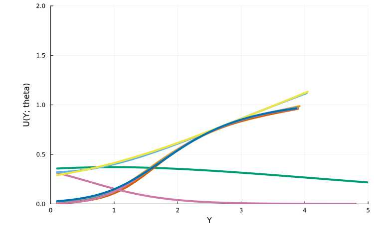
Ensemble plots are useful for practical functional identifiability analysis: if all runs converge to the same functional form, this suggests that only a single function is compatible with the data. By default, PEtab clusters the optimization runs as described here, and uses the cluster assignments to color the plotted functions.

To restrict the plot to well-fitting functions, use loss_thres to set an upper bound on the accepted loss value:

plot(
    petab_sol, petab_prob; plot_type = :function_ensemble,
    loss_thres = petab_sol.fmin + abs(petab_sol.fmin) / 2
)

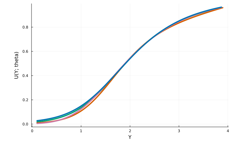
In this plot, all displayed functions are approximately Hill functions, consistent with the true activation function. Additional options for :function_ensemble:

• num_plotted_nn: number of functions to plot. Defaults to all functions meeting the loss_thres criterion.

• clustering_function: clustering function used to assign colors. Follows the same syntax as described here.

The :function_ensemble plot type also supports the plt_dens, nn_idx, plotted_dim, and x_support options available for :best_function. By default, PEtab infers the support separately for each plotted function.