SciML training strategies

Training SciML models that combine mechanistic ODEs and ML components is often challenging as methods that work well for pure ODE models (e.g. multi-start local optimization with quasi-Newton methods) often perform poorly. Moreover, ML-style training with the Adam optimizer for a fixed number of epochs is often insufficient. To address this, several training strategies have been developed, and via PEtabTraining.jl PEtab.jl supports three efficient ones: curriculum learning, multiple shooting, and curriculum multiple shooting.

This tutorial shows how to apply these three strategies and compare them to plain Adam optimization. It assumes familiarity with the SciML starter tutorial. As a running example, we fit a Neural ODE to time-series data generated from a Lotka–Volterra system.

using ComponentArrays, Lux, PEtab

function lv_node!(du, u, p, t, ml_models)
    prey, predator = u
    net1 = ml_models[:net1]
    nn_out, _ = net1.lux_model([prey, predator], p.net1, net1.st)
    du[1] = nn_out[1] # prey
    du[2] = nn_out[2] # predator
    return nothing
end

lux_model = Lux.Chain(
    Lux.Dense(2 => 5, Lux.swish),
    Lux.Dense(5 => 5, Lux.swish),
    Lux.Dense(5 => 2),
)
ml_model = MLModel(:net1, lux_model, false)

p_mechanistic = ComponentArray()
u0 = ComponentArray(prey = 0.44249296, predator = 4.6280594)
node_problem = UDEProblem(lv_node!, u0, (0.0, 10.0), p_mechanistic, ml_model)

parameters_est = [PEtabMLParameter(:net1)]

obs = [
    PEtabObservable(:obs_prey, :prey, 1.0),
    PEtabObservable(:obs_predator, :predator, 1.0),
]

Training and validation data are simulated from the mechanistic Lotka–Volterra model:

using DataFrames, StableRNGs, OrdinaryDiffEqTsit5
rng = StableRNGs.StableRNG(42)

function lv_ode!(du, u, p, t)
    prey, predator = u
    du[1] = p.alpha * prey - p.beta * prey * predator
    du[2] = p.gamma * prey * predator - p.delta * predator
    return nothing
end

u0 = [0.44249296, 4.6280594]
p_true = (alpha = 1.3, beta = 0.9, gamma = 0.8, delta = 1.8)
lv_prob = ODEProblem(lv_ode!, u0, (0.0, 13.0), p_true)
sol = solve(lv_prob, Tsit5(); abstol = 1e-8, reltol = 1e-8, saveat = 0:0.1:12.2)

obs_prey = sol[1, :] .+ 0.1 .* randn(rng, length(sol.t))
obs_predator = sol[2, :] .+ 0.1 .* randn(rng, length(sol.t))

df_prey = DataFrame(
    time = sol.t, measurement = obs_prey, obs_id = "obs_prey"
)
df_predator = DataFrame(
    time = sol.t, measurement = obs_predator, obs_id = "obs_predator"
)
df_m = vcat(df_prey, df_predator)

t_split = 6.1
df_train = filter(row -> row.time <= t_split, df_m)
df_val = filter(row -> row.time > t_split, df_m)

Plotting the training/validation split shows that this is a challenging training task due to the oscillatory dynamics:

using Plots
scatter(df_m.time, df_m.measurement, group = df_m.obs_id)
vline!(
    [t_split], label = "split train/validation", color = "black"
)

Given training/validation data, separate PEtabODEProblems can then be created for the training and validation objectives:

model_train = PEtabModel(
    node_problem, obs, df_train, parameters_est; ml_models = ml_model
)
model_val = PEtabModel(
    node_problem, obs, df_val, parameters_est; ml_models = ml_model
)
prob_train = PEtabODEProblem(model_train)
prob_val = PEtabODEProblem(model_val)

Generating starting points

Regardless of training strategy, optimization requires a start guess. For SciML problems (e.g. Neural ODEs/UDEs), training is typically more stable if the ML model is initialized with small weights and biases; otherwise the initial dynamics can be difficult to simulate. To this end, weight and bias initializers can be provided to get_startguesses:

rng = StableRNGs.StableRNG(12) # for reproducibility
# default is glorot_normal(; gain = 1.2)
x0 = get_startguesses(
    rng, prob_train, 1; init_bias = Lux.zeros64,
    init_weight = glorot_normal(; gain = 0.2),
)

To reduce sensitivity to local minima, it is often useful to try multiple random start guesses; but for simplicity, a single start guess is used in this tutorial.

Plain Adam training

As a baseline, we first train using Adam with a fixed learning rate. Given an initial guess, the objective and its gradient can be evaluated with prob_train.nllh(x) and prob_train.grad(x). These can then be used to implement a training loop:

using Optimisers

x = deepcopy(x0)
learning_rate = 1e-3
state = Optimisers.setup(Adam(learning_rate), x)

trace_adam = Float64[]
n_epochs = 6000
for epoch in 1:n_epochs
    g = prob_train.grad(x)
    state, x = Optimisers.update(state, x, g)

    # Stop if the objective cannot be evaluated (e.g. simulation failure)
    if !isfinite(prob_train.nllh(x))
        break
    end

    # Save training trace for plotting later
    if epoch % 25 == 0 || epoch == 1
        nllh = prob_train.nllh(x)
        push!(trace_adam, nllh)
    end
end

Plotting the fit shows an okay fit, but there is still clear room for improvement:

plot(x, prob_train)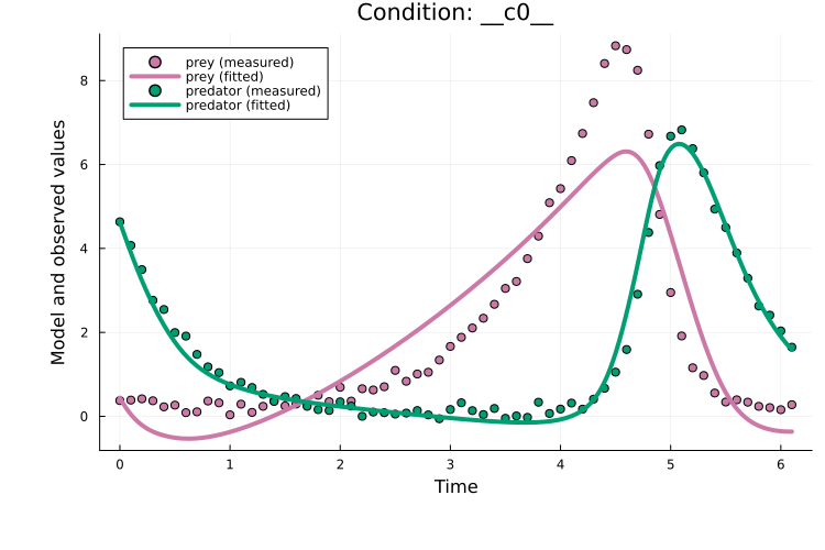

Training with plain Adam typically requires tuning two main hyperparameters besides the model architecture: the learning rate and the number of epochs. The required number of epochs is highly model-dependent. For the learning rate, 1e-3 is often a good starting point.

Curriculum learning

Curriculum learning is a strategy where problem difficulty is progressively increased across curriculum stages. For a PEtabODEProblem, this is done by starting from a subset of measurement time points and then gradually including more points until the full dataset is used.

With PEtabTraining.jl, as an example, a 5-stage curriculum problem can be created as:

using PEtabTraining
prob_cl = PEtabClProblem(prob_train, SplitTime(5))
describe(prob_cl)

PEtabClProblem UDEProblemModel
Problem statistics
  Parameters to estimate: 57
  ODE: 2 states, 57 parameters
  Observables: 2
  Simulation conditions: 1

Curriculum statistics (5 stages)
  Stage 1: tspan [0.0, 1.1]
           fraction (obs/cond): 1.0/1.0
  Stage 2: tspan [0.0, 2.3]
           fraction (obs/cond): 1.0/1.0
  Stage 3: tspan [0.0, 3.5]
           fraction (obs/cond): 1.0/1.0
  Stage 4: tspan [0.0, 4.7]
           fraction (obs/cond): 1.0/1.0
  Stage 5: tspan [0.0, 6.1]
           fraction (obs/cond): 1.0/1.0

describe(prob_cl) reports per-stage statistics (i.e. the fraction of observables and simulation conditions covered at each stage). As a rule of thumb, curriculum learning tends to work best when each stage includes most observables and conditions; otherwise the training objective changes too drastically between stages.

PEtabClProblem stores the stage problems in prob_cl.petab_problems as separate PEtabODEProblems, which can be used to write a training loop. For example:

using Optimisers

# Epoch ranges per stage
epochs_per_stage = [
    1 => 1:500, 2 => 501:1000, 3 => 1001:1500,
    4 => 1501:2000, 5 => 2001:6000,
]

x = deepcopy(x0)
learning_rate = 1e-3
state = Optimisers.setup(Adam(learning_rate), x)
trace_cl = Float64[]
for (stage, epochs) in epochs_per_stage
    prob_stage = prob_cl.petab_problems[stage]
    for epoch in epochs
        g = prob_stage.grad(x)
        state, x = Optimisers.update(state, x, g)

        # Stop if the objective cannot be evaluated (e.g. simulation failure)
        if !isfinite(prob_stage.nllh(x))
            break
        end

        # Save training trace (on full training objective for comparability)
        if epoch % 25 == 0 || epoch == 1
            push!(trace_cl, prob_train.nllh(x))
        end
    end
end

Plotting the fit shows that while more performant than pure Adam, training can still be improved:

plot(x, prob_train)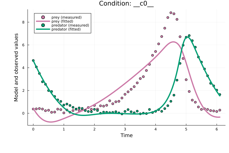

Curriculum learning introduces two additional tuning parameters compared to plain Adam: the number of stages and the epoch schedule per stage (epochs_per_stage above). Using curriculum for roughly the first third of training often works well. The number of stages is problem-dependent; 5 is a reasonable starting point, and using more stages often help if the problem has many measurements.

Multiple shooting

Multiple shooting is a strategy where the ODE simulation time span is split into windows that are fitted jointly. Each window has its own estimated initial state, and a (quadratic) continuity penalty is used to promote continuity between adjacent windows.

With PEtabTraining.jl, as an example, a 5-window problem can be created as:

using PEtabTraining
prob_ms = PEtabMsProblem(prob_train, SplitTime(5))
describe(prob_ms)

PEtabMsProblem UDEProblemModel
Problem statistics
  Parameters to estimate: 57
  ODE: 2 states, 57 parameters
  Observables: 2
  Simulation conditions: 1

Window statistics (5 windows)
  Penalty λ = 1.0e+00, window u0 parameters: 8
  Window 1: tspan [0.0, 1.2]
  Window 2: tspan [1.2, 2.4]
  Window 3: tspan [2.4, 3.6]
  Window 4: tspan [3.6, 4.8]
  Window 5: tspan [4.8, 6.1]

Here, describe(prob_ms) reports each window time span and the default quadratic penalty.

Two key tuning parameters for multiple shooting are the window penalty and the initialization of window initial states. Initializing window states to small values (e.g. 0.1) often works well, while the penalty typically needs tuning. Both can be set with:

# Set penalty to 100
set_ms_window_penalty!(prob_ms, 100.0)
# Set initial window value
prob_ms_train = prob_ms.petab_ms_problem
x_ms = get_x(prob_ms_train)
set_u0_ms_windows!(x_ms, prob_ms; init = MsInitConstant(0.01))

Note that prob_ms_train is a PEtabODEProblem corresponding to a multiple-shooting rewrite of the original problem. With it, a training loop can be written as:

x_ms[keys(x0)] .= x0
learning_rate = 1e-3
state = Optimisers.setup(Adam(learning_rate), x_ms)
trace_ms = Float64[]
for epoch in 1:n_epochs
    g = prob_ms_train.grad(x_ms)
    state, x_ms = Optimisers.update(state, x_ms, g)

    # Stop if the objective cannot be evaluated (e.g. simulation failure)
    if !isfinite(prob_ms_train.nllh(x_ms))
        break
    end

    # Save training trace, for the targeted original train problem
    if epoch % 25 == 0 || epoch == 1
        x = x_ms[keys(x0)]
        push!(trace_ms, prob_train.nllh(x))
    end
end

In the example above, keys(x0) maps between the original parameter vector (x0) and the multiple-shooting parameter vector (x_ms). Since multiple shooting also estimates window initial states, x_ms has additional entries and therefore a different dimension than x0. Because the vectors are ComponentArrays, shared parameters can be copied between them by indexing by name, as above.

Plotting the fit shows that, for this example, multiple shooting does improves over plain Adam:

x = x_ms[keys(x0)]
plot(x, prob_train)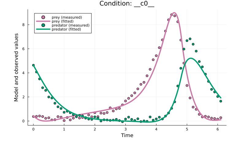

Multiple shooting introduces two additional tuning parameters compared to plain Adam: the number of windows and the window penalty. Both can be tricky to tune; so while well-tuned multiple shooting can be highly effective, it can be non-trivial to achieve in practice. Moreover, since this approach estimates a separate initial values for each window, it can perform poorly for partially observed systems. Curriculum multiple shooting addresses these limitations by combining multiple shooting with a curriculum schedule.

Curriculum multiple shooting

Curriculum multiple shooting combines multiple shooting with a curriculum schedule. Training starts from a multiple-shooting formulation and progressively reduces the number of windows by merging adjacent windows until the original single-window problem is recovered.

With PEtabTraining.jl, as an example, a 5-stage curriculum multiple-shooting problem can be created as:

using PEtabTraining
prob_cl_ms = PEtabClMsProblem(prob_train, SplitTime(5))
describe(prob_cl_ms)

PEtabClMsProblem UDEProblemModel
Problem statistics
  Parameters to estimate: 57
  ODE: 2 states, 57 parameters
  Observables: 2
  Simulation conditions: 1

Curriculum statistics (5 stages)
  Window penalty λ = 1.0e+00
  Stage 1: window tspans [0, 1.2], [1.2, 2.4], [2.4, 3.6], [3.6, 4.8], [4.8, 6.1]
  Stage 2: window tspans [0, 2.4], [1.2, 3.6], [2.4, 4.8], [3.6, 6.1]
  Stage 3: window tspans [0, 3.6], [1.2, 4.8], [2.4, 6.1]
  Stage 4: window tspans [0, 4.8], [1.2, 6.1]
  Stage 5: original problem

describe(prob_cl_ms) reports per-stage window ranges and the default window quadratic continuity penalty. As for multiple shooting, two key tuning parameters are the window penalty and the initialization of window initial states. Both can be set with:

# Window penalty
set_ms_window_penalty!(prob_cl_ms, 1.0)
# Initialize window states for stage 1
x_cl_ms = get_x(prob_cl_ms.petab_problems[1])
set_u0_ms_windows!(x_cl_ms, prob_cl_ms, 1; init = MsInitConstant(0.01))

PEtabClMsProblem stores the stage problems in prob_cl_ms.petab_problems as separate PEtabODEProblems, which can be used to write a training loop. When moving between stages, map_x_stage maps parameters to the next stage (the window count changes, so the window initial states must be remapped). For example:

using Optimisers

epochs_per_stage = [
    1 => 1:500, 2 => 501:1000, 3 => 1001:1500,
    4 => 1501:2000, 5 => 2001:6000,
]

x_cl_ms[keys(x0)] .= x0
trace_cl_ms = Float64[]
for (stage, epochs) in epochs_per_stage
    if stage > 1
        x_cl_ms = map_x_stage(x_cl_ms, prob_cl_ms, stage - 1, stage)
    end

    prob_stage = prob_cl_ms.petab_problems[stage]
    state = Optimisers.setup(Adam(learning_rate), x_cl_ms)

    for epoch in epochs
        g = prob_stage.grad(x_cl_ms)
        state, x_cl_ms = Optimisers.update(state, x_cl_ms, g)

        # Stop if the objective cannot be evaluated (e.g. simulation failure)
        if !isfinite(prob_stage.nllh(x_cl_ms))
            break
        end

        # Save training trace on the original training objective for comparability
        if epoch % 25 == 0 || epoch == 1
            x = x_cl_ms[keys(x0)]
            push!(trace_cl_ms, prob_train.nllh(x))
        end
    end
end

Plotting the fit shows that curriculum multiple shooting clearly improves over plain Adam:

x = x_cl_ms[keys(x0)]
plot(x, prob_train)
title!("Training data")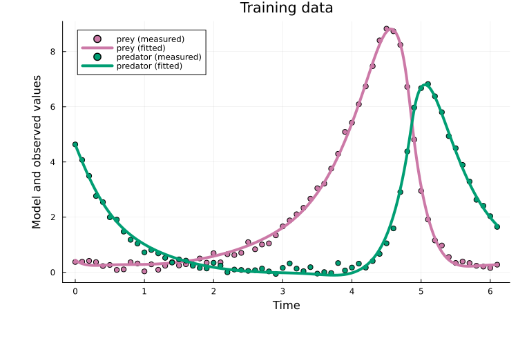

It also generalizes well to the validation data:

plot(x, prob_val)
title!("Validation data")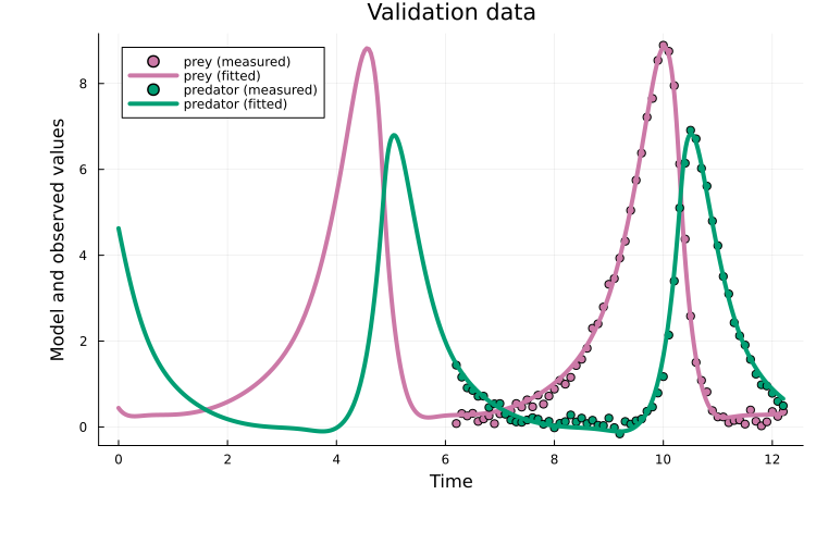

Curriculum multiple shooting introduces three additional tuning parameters compared to plain Adam: the number of stages, the epoch schedule per stage (epochs_per_stage above), and the window penalty. In practice, the stage schedule and number of stages can be tuned similarly to curriculum learning. The window penalty typically still requires tuning, but compared to multiple shooting this approach is often more robust.

Comparing approaches

Plotting the training traces shows that, for this example, curriculum multiple shooting performs best:

using Plots
x_vals = vcat(1, 25:25:n_epochs)
plot(x_vals, trace_adam, label = "Adam", yaxis = :log10)
plot!(x_vals, trace_cl, label = "CL")
plot!(x_vals, trace_ms, label = "MS")
plot!(x_vals, trace_cl_ms, label = "CL + MS")
xlabel!("Epoch"); ylabel!("NLLH")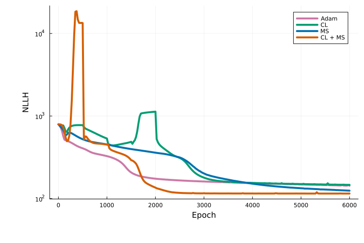

It should be kept in mind that this comparison is based on a single run for a single model. An extensive benchmark study to evaluate these approaches is in progress.

Next steps

More details on available options for each training strategy are provided in the PEtabTraining.jl documentation.

The training strategies covered here can also be used for mechanistic models. For example, curriculum training can be combined with the Fides.jl optimizer via calibrate to optimize a mechanistic model in stages, which can be highly effective. More tutorials on this are coming, so stay tuned!