Parameter estimation tutorial

A PEtabODEProblem provides runtime-efficient objective, gradient, and (optionally) Hessian functions for estimating unknown model parameters with numerical optimization algorithms. Specifically, the parameter-estimation problem targeted is

$$\underset{\mathbf{x}\in {\mathbb{R}}^N}{min}-\ell (\mathbf{x})\text{subject to}\mathbf{lb}\le \mathbf{x}\le \mathbf{ub},$$

where -ℓ(x) is a negative log-likelihood (see PEtabObservable for mathematical definition) and lb/ub are parameter bounds.

This extended tutorial covers PEtab.jl’s single-start and multi-start parameter estimation workflows. It also shows how to construct an OptimizationProblem to solve the problem using the Optimization.jl interface. As a running example, we use the Michaelis–Menten model from the starting tutorial.

using Catalyst, PEtab
rn = @reaction_network begin
    @parameters S0 c3=3.0
    @species begin
        S(t) = S0
        E(t) = 50.0
        SE(t) = 0.0
        P(t) = 0.0
    end
    @observables begin
        obs1 ~ S + E
        obs2 ~ P
    end
    c1, S + E --> SE
    c2, SE --> S + E
    c3, SE --> P + E
end

# Observables
@parameters sigma
petab_obs1 = PEtabObservable(:petab_obs1, :obs1, 3.0)
petab_obs2 = PEtabObservable(:petab_obs2, :obs2, sigma)
observables = [petab_obs1, petab_obs2]

# Parameters to estimate
p_c1 = PEtabParameter(:c1)
p_c2 = PEtabParameter(:c2)
p_S0 = PEtabParameter(:S0)
p_sigma = PEtabParameter(:sigma)
pest = [p_c1, p_c2, p_S0, p_sigma]

# Measurements; simulate with 'true' parameters
using DataFrames, OrdinaryDiffEqRosenbrock
ps = [:c1 => 1.0, :c2 => 10.0, :c3 => 1.0, :S0 => 100.0]
u0 = [:S => 100.0, :E => 50.0, :SE => 0.0, :P => 0.0]
tspan = (0.0, 10.0)
oprob = ODEProblem(rn, u0, tspan, ps)
sol = solve(oprob, Rodas5P(); saveat = 0:0.5:10.0)
obs1 = (sol[:S] + sol[:E]) .+ randn(length(sol[:E]))
obs2   = sol[:P] .+ randn(length(sol[:P]))
df1 = DataFrame(obs_id = "petab_obs1", time = sol.t, measurement = obs1)
df2 = DataFrame(obs_id = "petab_obs2", time = sol.t, measurement = obs2)
measurements = vcat(df1, df2)

# Create the PEtabODEProblem
petab_model = PEtabModel(rn, observables, measurements, pest)
petab_prob = PEtabODEProblem(petab_model)

Single-start parameter estimation

Single-start parameter estimation runs a local optimizer from an initial parameter vector x0. In PEtab.jl, parameters must be provided in the internal order expected by the objective. The easiest way to construct a correctly ordered start vector is get_x:

x0 = get_x(petab_prob)

ComponentVector{Float64}(log10_c1 = 2.6989704386302837, log10_c2 = 2.6989704386302837, log10_S0 = 2.6989704386302837, log10_sigma = 2.6989704386302837)

x0 is a ComponentArray, so parameters can be accessed by name. Names are also prefixed by parameter scale, and by default parameters are estimated on a log10 scale as it often improves estimation performance [3, 4]. Values should be modified on the estimation scale:

x0.log10_c1 = log10(10.0)
x0[:log10_c1] = log10(10.0) # alternatively

Given a starting point, single-start parameter estimation can be performed with calibrate:

PEtab.calibrate Function

calibrate(prob::PEtabODEProblem, x0, alg; kwargs...)::PEtabOptimisationResult

From starting point x0 using optimization algorithm alg, estimate unknown model parameters for prob, and get results as a PEtabOptimisationResult.

x0 can be a Vector or a ComponentArray, where the individual parameters must be in the order expected by prob. To get a vector in the correct order, see get_x.

A list of available and recommended optimization algorithms (alg) can be found in the documentation. Briefly, supported algorithms are from:

• Optim.jl: LBFGS(), BFGS(), or IPNewton() methods.

• Ipopt.jl: IpoptOptimizer() interior-point Newton method.

• Fides.jl: Newton trust region for box-constrained problem. Fides can either use the Hessian in prob (alg = Fides.CustomHessian()), or any of its built in Hessian approximations (e.g. alg = Fides.BFGS()). A full list of Hessian approximations can be found in the Fides documentation

Different ways to visualize the parameter estimation result can be found in the documentation.

See also PEtabOptimisationResult and IpoptOptimizer

Keyword Arguments

• save_trace::Bool = false: Whether to save the optimization trace of the objective function and parameter vector. Only applicable for some algorithms; see the documentation for details.

• options = DEFAULT_OPTIONS: Configurable options for alg. The type and available options depend on which package alg belongs to. For example, if alg = IPNewton() from Optim.jl, options should be provided as an Optim.Options() struct. A list of configurable options can be found in the documentation.

source

Algorithm recommendations are summarized on Optimizer options. Following those recommendations, we use Optim.jl’s interior-point Newton method:

import Optim
res = calibrate(petab_prob, x0, Optim.IPNewton())

PEtabOptimisationResult
  min(f)                = 1.54e+02
  Parameters estimated  = 4
  Optimiser iterations  = 23
  Runtime               = 1.4e+00s
  Optimiser algorithm   = Optim_IPNewton

calibrate returns a PEtabOptimisationResult containing the optimized parameters and common diagnostics. To visualize the fit and other diagnostics, see Plotting optimization results. For example, the model fit can be plotted with:

using Plots
plot(res, petab_prob)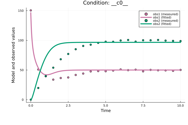

A major drawback of single-start estimation is that it may converge to a local minimum. A better strategy for finding the global minimum is multi-start parameter estimation.

Multi-start parameter estimation

Multi-start parameter estimation runs a local optimizer from multiple randomly sampled starting points. This approach empirically performs well for ODE models [1, 3].

The first step is to generate n starting points within the parameter bounds. Pure random sampling tends to cluster, so PEtab.jl supports quasi-Monte Carlo sampling (Latin hypercube by default), which typically gives more space-filling points that improves estimation performance [3]:

using Distributions, QuasiMonteCarlo, Plots
lb, ub = [-1.0, -1.0], [1.0, 1.0]
s_uniform = QuasiMonteCarlo.sample(100, lb, ub, Uniform())
s_lhs     = QuasiMonteCarlo.sample(100, lb, ub, LatinHypercubeSample())
p1 = plot(
    s_uniform[1, :], s_uniform[2, :]; title = "Uniform sampling",
    seriestype = :scatter, label = false
)
p2 = plot(
    s_lhs[1, :], s_lhs[2, :]; title = "Hypercube sampling",
    seriestype=:scatter, label=false)
plot(p1, p2)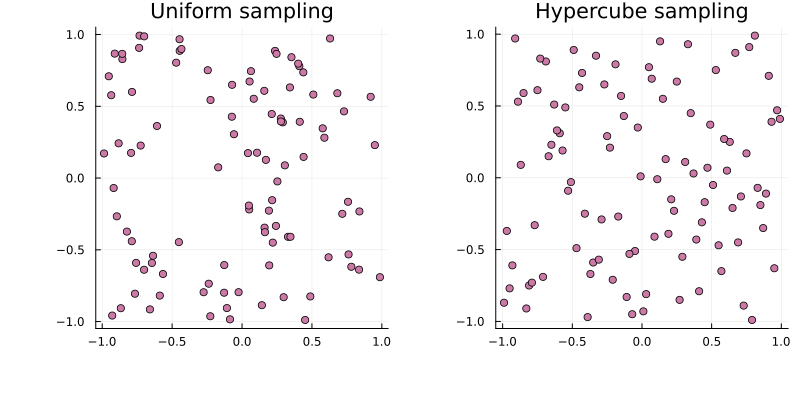

For a PEtabODEProblem, hypercube start guesses (respecting bounds and parameter scales) can be generated with get_startguesses:

using StableRNGs
rng = StableRNG(42)
x0s = get_startguesses(rng, petab_prob, 50)

Given x0s, multi-start estimation can be performed by calling calibrate repeatedly. For convenience, calibrate_multistart combines start-guess generation and estimation:

PEtab.calibrate_multistart Function

calibrate_multistart([rng::AbstractRng], prob::PEtabODEProblem, alg, nmultistarts::Integer;
                     nprocs = 1, dirsave=nothing, kwargs...)::PEtabMultistartResult

Perform nmultistarts parameter estimation runs from randomly sampled starting points using the optimization algorithm alg to estimate the unknown model parameters in prob.

A list of available and recommended optimisation algorithms (alg) can be found in the package documentation and in the calibrate documentation.

As with get_startguesses, the rng controlling the generation of starting points is optional; if omitted, Random.default_rng() is used. For reproducible starting points, pass a seeded rng (e.g., MersenneTwister(42)).

If nprocs > 1, the parameter estimation runs are performed in parallel using the pmap function from Distributed.jl with nprocs processes. If parameter estimation on a single process (nprocs = 1) takes longer than 5 minutes, we strongly recommend setting nprocs > 1, as this can greatly reduce runtime. Note that nprocs should not be larger than the number of cores on the computer.

If dirsave is provided, intermediate results for each run are saved in dirsave. It is strongly recommended to provide dirsave for larger models, as parameter estimation can take hours (or even days!),and without dirsave, all intermediate results will be lost if something goes wrong.

Different ways to visualize the parameter estimation result can be found in the documentation.

See also PEtabMultistartResult, get_startguesses, and calibrate.

Keyword Arguments

• sampling_method = LatinHypercubeSample(): Method for sampling a diverse (spread out) set of starting points. See the documentation for get_startguesses, which is the function used for generating starting points.

• sample_prior::Bool = true: See the documentation for get_startguesses.

• options = DEFAULT_OPTIONS: Configurable options for alg. See the documentation for calibrate.

source

Two important keyword arguments to calibrate_multistart are nprocs and dirsave. nprocs controls how many runs are executed in parallel (via pmap from Distributed.jl). Using nprocs > 1 often reduces wall-clock time for problems taking >5 minutes. dirsave optionally saves results as runs finish and is strongly recommended to not loose intermediate results. For example, to run 50 multi-starts with Optim.jl’s IPNewton:

ms_res = calibrate_multistart(
  petab_prob, Optim.IPNewton(), 50; nprocs = 2,
  dirsave = "path_to_save_directory"
)

PEtabMultistartResult
  min(f)                = 1.54e+02
  Parameters estimated  = 4
  Number of multistarts = 50
  Optimiser algorithm   = Optim_IPNewton
  Results saved at path_to_save_directory

Results are returned as a PEtabMultistartResult, which contains per-run statistics and the best solution. Different ways to visualize results are found in Plotting optimization results. A common diagnostic is a waterfall plot of the final objective values across runs:

plot(ms_res; plot_type=:waterfall)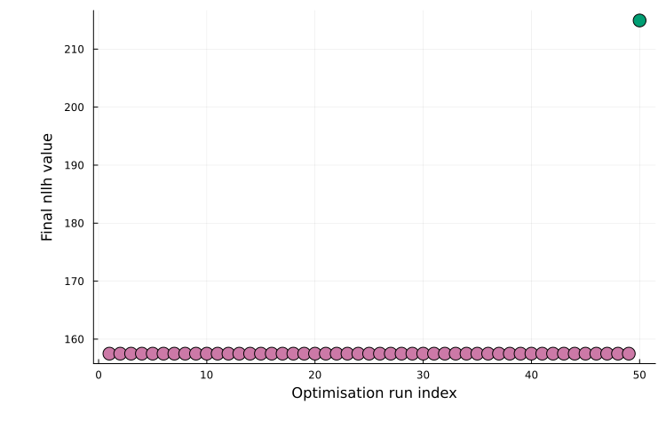

Plateaus typically indicate distinct local optima (multiple runs converging to similar final objective values). As another example, the best model fit can be plotted as:

plot(ms_res, petab_prob)

Creating an OptimizationProblem

Optimization.jl provides a unified interface to many optimization libraries (100+ solvers across 25+ packages). Since the Optimization.jl ecosystem is still evolving, some PEtab.jl convenience features (e.g. plotting of multi-start estimation results) are not yet available when using Optimization.jl directly. We therefore recommend the PEtab.jl wrappers as the default workflow, but this is likely to change as Optimization.jl matures.

A PEtabODEProblem can be converted directly into an OptimizationProblem:

PEtab.OptimizationProblem Function

OptimizationProblem(prob::PEtabODEProblem; box_constraints::Bool = true)

Create an Optimization.jl OptimizationProblem from prob.

To use algorithms not compatible with box constraints (e.g., Optim.jl NewtonTrustRegion), set box_constraints = false. Note that with this option, optimizers may move outside the bounds, which can negatively impact performance. More information on how to use an OptimizationProblem can be found in the Optimization.jl documentation.

source

For our working example:

using Optimization
opt_prob = OptimizationProblem(petab_prob)

OptimizationProblem. In-place: true
u0: ComponentVector{Float64}(log10_c1 = 1.0, log10_c2 = 2.6989704386302837, log10_S0 = 2.6989704386302837, log10_sigma = 2.6989704386302837)

Given a start guess x0, parameters can be estimated with any supported solver. For example, using Optim.jl’s ParticleSwarm() via OptimizationOptimJL:

using OptimizationOptimJL
opt_prob.u0 .= x0
res = solve(opt_prob, Optim.ParticleSwarm())

retcode: Failure
u: ComponentVector{Float64}(log10_c1 = -1.0418879498351266, log10_c2 = -3.0, log10_S0 = 1.9835996663597477, log10_sigma = 1.1308418011544303)

solve returns an OptimizationSolution. For solver options and how to work with the returned solution object, see the Optimization.jl documentation.

Next steps

This extended tutorial showed how to estimate parameters with PEtab.jl. The parameter estimation tutorials also covers:

• Available optimization algorithms: Supported and recommended algorithms.

• Plotting parameter estimation results: Plotting options for parameter estimation output.

• Wrapping optimization packages: How to use a PEtabODEProblem directly with an optimization package such as Optim.jl.

• Model selection (PEtab-select): Automatic model selection with PEtab-Select [11].

• Litterature references: Good introductions on parameter estimation for ODE models can be found in [3, 12].

References

1. S. Persson, F. Fröhlich, S. Grein, T. Loman, D. Ognissanti, V. Hasselgren, J. Hasenauer and M. Cvijovic. PEtab. jl: advancing the efficiency and utility of dynamic modelling. Bioinformatics 41, btaf497 (2025).

2. A. Raue, M. Schilling, J. Bachmann, A. Matteson, M. Schelke, D. Kaschek, S. Hug, C. Kreutz, B. D. Harms, F. J. Theis and others. Lessons learned from quantitative dynamical modeling in systems biology. PloS one 8, e74335 (2013).

3. H. Hass, C. Loos, E. Raimundez-Alvarez, J. Timmer, J. Hasenauer and C. Kreutz. Benchmark problems for dynamic modeling of intracellular processes. Bioinformatics 35, 3073–3082 (2019).

4. D. Pathirana, F. T. Bergmann, D. Doresic, P. Lakrisenko, S. Persson, N. Neubrand, J. Timmer, C. Kreutz, H. Binder, M. Cvijovic and others. PEtab Select: specification standard and supporting software for automated model selection, bioRxiv, 2025–05 (2025).

5. A. F. Villaverde, D. Pathirana, F. Fröhlich, J. Hasenauer and J. R. Banga. A protocol for dynamic model calibration. Briefings in bioinformatics 23, bbab387 (2022).