Bayesian inference
PEtab.jl’s parameter-estimation workflow is frequentist and targets a maximum-likelihood (or maximum a posteriori, when priors are included) estimate. When prior knowledge about the parameters is available, Bayesian inference offers an alternative approach to model fitting by inferring the posterior distribution of the parameters given data,
Adaptive Metropolis–Hastings samplers from AdaptiveMCMC.jl [18].
Hamiltonian Monte Carlo (HMC) samplers from AdvancedHMC.jl, including NUTS as in Stan [19, 20].
This tutorial shows how to (i) define priors in a PEtabODEProblem, and (ii) run Bayesian inference with AdaptiveMCMC.jl and AdvancedHMC.jl. Note that this functionality is planned to move into a separate package, and the API will change in the future.
INFO
To use Bayesian inference functionality, load Bijectors.jl, LogDensityProblems.jl, and LogDensityProblemsAD.jl.
Creating a Bayesian inference problem
For PEtab problems in the PEtab standard format, priors are defined in the parameter table. Here, we instead consider a model defined directly in Julia: a simple saturated growth model. First, let’s define the model and simulate data:
using DataFrames, Distributions, OrdinaryDiffEqRosenbrock,
    ModelingToolkitBase, PEtab, Plots
using ModelingToolkitBase: t_nounits as t, D_nounits as D

ps = @parameters b1 b2
sps = @variables x(t) = 0.0 obs_x(t)
eqs = [
    # Dynamics
    D(x) ~ b2 * (b1 - x)
    # Observables
    obs_x ~ x
]
@named sys_model = System(eqs, t, sps, ps)
sys = mtkcompile(sys_model)

# Simulate data with Normal measurement noise (σ = 0.03)
oprob = ODEProblem(sys, [0.0], (0.0, 2.5), [1.0, 0.2])
tsave = range(0.0, 2.5, 101)
sol = solve(oprob, Rodas5P(); abstol=1e-12, reltol=1e-12, saveat=tsave)
obs = sol[:x] .+ rand(Normal(0.0, 0.03), length(tsave))
measurements = DataFrame(obs_id="obs_x", time=sol.t, measurement=obs)

# Observable
@parameters sigma
observables = PEtabObservable(:obs_x, :obs_x, sigma)

# Plot the data
plot(measurements.time, measurements.measurement; seriestype=:scatter,
    title="Observed data")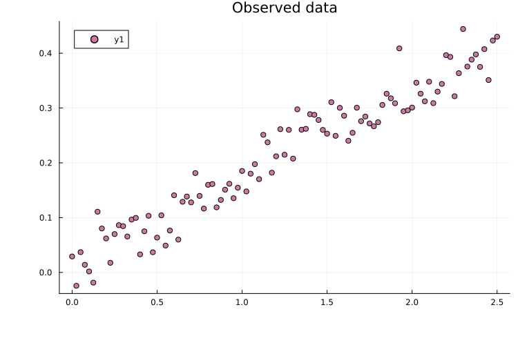
Priors are assigned via PEtabParameter using any continuous distribution from Distributions.jl. For example:
pest = [
    PEtabParameter(:b1, value=1.0, scale=:lin, prior=Uniform(0.0, 5.0)),
    PEtabParameter(:b2, value=0.2, prior=LogNormal(1.0, 1.0)),
    PEtabParameter(:sigma, value=0.03, scale=:lin, prior=Gamma(1.0, 1.0))
]
3-element Vector{PEtabParameter}:
PEtabParameter b1: estimate (scale = lin, prior(b1) = Uniform(a=0.0, b=5.0))
PEtabParameter b2: estimate (scale = log10, prior(b2) = LogNormal(μ=1.0, σ=1.0))
PEtabParameter sigma: estimate (scale = lin, prior(sigma) = Gamma(α=1.0, θ=1.0))Priors are evaluated on the parameter’s linear (non-transformed) scale. For example, while b2 above is estimated on the log10 scale, the prior applies to b1 (not log10(b1)). If no prior is provided, the default is a Uniform over the parameter bounds. Finally, build the problem as usual:
model = PEtabModel(sys, observables, measurements, pest)
petab_prob = PEtabODEProblem(model)
PEtabODEProblem ODESystemModel: 3 parameters to estimate
(for more statistics, call `describe(petab_prob)`)Bayesian inference (general setup)
To run Bayesian inference, first construct a PEtabLogDensity. This object implements the LogDensityProblems.jl interface and can be used as the target density for MCMC:
using Bijectors, LogDensityProblems, LogDensityProblemsAD
target = PEtabLogDensity(petab_prob)
PEtabLogDensity with 3 parameters to inferODE-solver and derivative settings are taken from petab_prob (here, the default gradient method :ForwardDiff and the Rodas5P solver).
A key choice is the starting point. For simplicity, we start from the nominal parameter vector, but in practice inference should be run with multiple chains and dispersed starting points [21]:
x = get_x(petab_prob)It is important to note that inference in PEtab.jl is performed on an unconstrained inference scale, since many inference algorithms (e.g. NUTS) operate on Uniform(0.0, 5.0)) are mapped to x (on parameter scale), inference uses the composition x -> x_prior -> x_inference:
x_prior = to_prior_scale(petab_prob.xnominal_transformed, target)
x_inference = target.inference_info.bijectors(x_prior)
3-element Vector{Float64}:
-1.3862943611198906
-1.6094379124341003
-3.506557897319982Inference results are then reported back on the prior scale with the to_chains function (see below).
WARNING
The initial value passed to the sampler must be on the inference scale (x_inference).
Bayesian inference with AdvancedHMC.jl (NUTS)
Given a starting point, NUTS can be run with 2000 samples and 1000 adaptation steps via:
using AdvancedHMC
# δ = 0.8 is the target acceptance rate (default in Stan)
sampler = NUTS(0.8)
res = sample(
    target, sampler, 2000; n_adapts = 1000, initial_params = x_inference,
    drop_warmup = true, progress = false,
)
[ Info: Found initial step size 0.0125Any sampler supported by AdvancedHMC.jl can be used (see the documentation). To work with results using a standard interface, convert to an MCMCChains.Chains:
using MCMCChains
chain_hmc = PEtab.to_chains(res, target)
Chains MCMC chain (2000×3×1 Array{Float64, 3}):
Iterations = 1:1:2000
Number of chains = 1
Samples per chain = 2000
parameters = b1, b2, sigma
Use `describe(chains)` for summary statistics and quantiles.This can be plotted with:
using Plots, StatsPlots
plot(chain_hmc)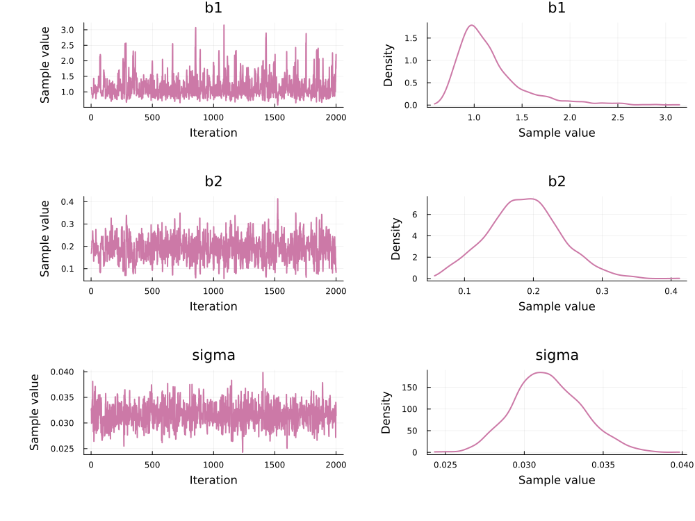
INFO
PEtab.to_chains converts samples back to the prior (linear) scale (not the unconstrained inference scale).
Bayesian inference with AdaptiveMCMC.jl
Given a starting point, the robst adaptive random-walk Metropolis sampler can be run for
using AdaptiveMCMC
# target.logtarget is the posterior log density on the inference scale
res = adaptive_rwm(x_inference, target.logtarget, 100000; progress=false)
Convert the result to an MCMCChains.Chains:
using MCMCChains, Plots, StatsPlots
chain_adapt = PEtab.to_chains(res, target)
plot(chain_adapt)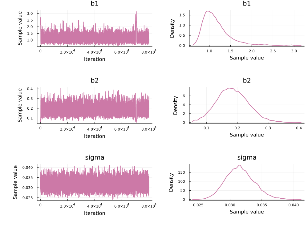
Other samplers from AdaptiveMCMC.jl can be used; see the documentation.
References
M. Vihola. Ergonomic and reliable Bayesian inference with adaptive Markov chain Monte Carlo. Wiley statsRef: statistics reference online, 1–12 (2014).
M. D. Hoffman, A. Gelman and others. The No-U-Turn sampler: adaptively setting path lengths in Hamiltonian Monte Carlo. J. Mach. Learn. Res. 15, 1593–1623 (2014).
B. Carpenter, A. Gelman, M. D. Hoffman, D. Lee, B. Goodrich, M. Betancourt, M. A. Brubaker, J. Guo, P. Li and A. Riddell. Stan: A probabilistic programming language. Journal of statistical software 76 (2017).
A. Gelman, A. Vehtari, D. Simpson, C. C. Margossian, B. Carpenter, Y. Yao, L. Kennedy, J. Gabry, P.-C. Bürkner and M. Modrák. Bayesian workflow, arXiv preprint arXiv:2011.01808 (2020).