Plotting parameter estimation results
After parameter estimation, plotting the results can help evaluate:
whether the model fits the data,
whether better-fitting parameter sets were missed (suggesting convergence to a local minimum), and
whether multiple distinct parameter sets fit the data equally well (suggesting a parameter identifiability issue).
In PEtab.jl, these plots are generated by calling plot on the output of calibrate (PEtabOptimisationResult) or calibrate_multistart (PEtabMultistartResult), using plot_type to select the plot. This tutorial covers the two broad plot types implemented:
Optimization diagnostics (e.g. objective values, parameter values across runs).
Model fit diagnostics (agreement between simulations and measured data).
Optimization diagnostics
As a working example, this section uses pre-computed parameter estimation results from a published model loaded into a PEtabMultistartResult (files can be downloaded here):
using PEtab, Plots
# path_res depends on where result is stored
ms_res = PEtabMultistartResult(path_res)
Objective function evaluation plot
The objective-evaluation plot is generated with plot_type = :objective and is available for both single-start and multi-start results. It shows the objective value at each optimizer iteration. For single-start estimation, a single trajectory is shown; for multi-start estimation, each run produces one trajectory.
plot(ms_res; plot_type = :objective)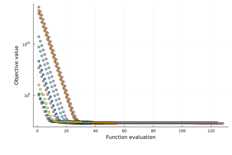
If the objective cannot be evaluated for a parameter set (e.g. simulation failure), the corresponding points are marked with crosses.
For multi-start plots, runs are colored by a clustering procedure that groups runs converging to the same local minimum (details and tunable options are documented here). When many runs are performed, the plot can become cluttered, therefore only the 10 best runs are shown (can be customized).
y-axis scale
For plot_type = :objective (as well as :best_objective, :waterfall, and :runtime_eval), PEtab.jl automatically chooses a linear or logarithmic y-axis. These defaults can be overridden with yaxis_scale and obj_shift.
Best objective value plot
The best-objective plot is generated with plot_type = :best_objective and is available for both single-start and multi-start results. It is similar to the objective-evaluation plot, but shows the best value reached so far at each iteration (and is therefore non-increasing). This is the default for single-start parameter estimation.
plot(ms_res; plot_type = :best_objective)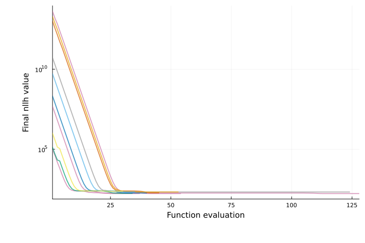
Waterfall plot
The waterfall plot is generated with plot_type = :waterfall and is only available for multi-start results. It shows the final objective value for each run, sorted from best to worst. Local minima often appear as plateaus, and runs with similar final objective values are grouped by color.
plot(ms_res; plot_type = :waterfall)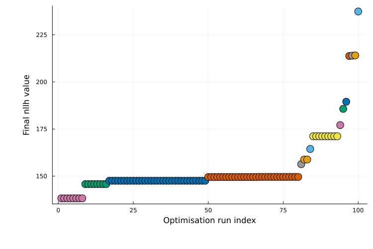
This is the default plot type for multi-start results. For additional guidance on interpretation, see Fig. 5 in [3].
Parallel coordinates plot
The parallel coordinates plot is generated with plot_type = :parallel_coordinates and is available for multi-start results. It visualizes parameter values for the best runs, with each run shown as a line. Parameter values are normalized per parameter: 0 corresponds to the minimum value observed and 1 to the maximum.
Runs with similar lines typically converged to the same local minimum. If runs with similar objective values show widely different values for a parameter, it suggests that the parameter is unidentifiable (i.e. multiple values yield equally good fits).
plot(ms_res; plot_type = :parallel_coordinates)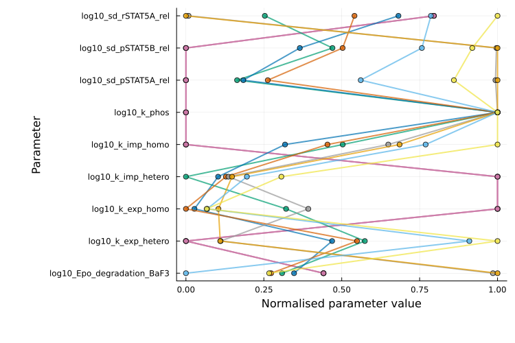
Runtime evaluation plots
The runtime-evaluation plot is generated with plot_type = :runtime_eval and is only available for multi-start results. It is a scatter plot showing runtime versus final objective value for each run:
plot(ms_res; plot_type = :runtime_eval)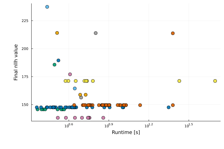
Multi-start run color clustering
For multi-start results (e.g. from calibrate_multistart), plots can contain many runs. By default, PEtab.jl applies a clustering step to group runs that likely converged to the same local minimum; runs in the same cluster are shown with the same color.
The default method is objective_value_clustering, which assigns the same cluster to runs whose final objective values differ by at most 0.1. A custom clustering method can be passed to plot via the clustering_function keyword argument. The function should have signature
input:
Vector{PEtabOptimisationResult}output:
Vector{Int}of the same length, with one cluster label per run.
Sub-selecting runs to plot
For multi-start results, plots such as :objective, :best_objective, and :parallel_coordinates can become cluttered when many runs are present. By default, these plot types show only the 10 runs with the best final objective values. This behavior can be changed with two keywords:
best_idxs_n::Int: number of top runs to include (starting from the best).idxs: explicit indices of runs to plot.
For :waterfall and :runtime_eval, all runs are shown by default, but best_idxs_n and idxs can still be used to restrict the plotted runs.
Model fit diagnostics
Simulation output against data (e.g., model fit and residuals) can be evaluated by passing the optimization result and the PEtabODEProblem to plot. By default, model-fit plots show all observables for the first simulation condition; this can be modified via the observable_ids and to condition keywords (see below).
As a working example, this section uses the Michaelis–Menten enzyme kinetics model from the starting tutorial, fitted to two simulation conditions (cond1, cond2) and two observables (obs_e, obs_p).
using Catalyst
rn = @reaction_network begin
    @species E(t)=1.0 SE(t)=0.0 P(t)=0.0
    kB, S + E --> SE
    kD, SE --> S + E
    kP, SE --> P + E
end
u0 = [:E => 1.0, :SE => 0.0, :P => 0.0]
p_true = [:kB => 1.0, :kD => 0.1, :kP => 0.5]

# Simulate data
using OrdinaryDiffEqRosenbrock
# cond1
oprob_true_cond1 = ODEProblem(rn, [:S => 1.0; u0], (0.0, 10.0), p_true)
true_sol_cond1 = solve(oprob_true_cond1, Rodas5P())
data_sol_cond1 = solve(oprob_true_cond1, Rodas5P(); saveat=1.0)
cond1_t = data_sol_cond1.t[2:end]
cond1_e = (0.8 .+ 0.1*randn(10)) .* data_sol_cond1[:E][2:end]
cond1_p = (0.8 .+ 0.1*randn(10)) .* data_sol_cond1[:P][2:end]
# cond2
oprob_true_cond2 = ODEProblem(rn, [:S => 0.5; u0], (0.0, 10.0), p_true)
true_sol_cond2 = solve(oprob_true_cond2, Rodas5P())
data_sol_cond2 = solve(oprob_true_cond2, Rodas5P(); saveat=1.0)
cond2_t = data_sol_cond2.t[2:end]
cond2_e = (0.8 .+ 0.1*randn(10)) .* data_sol_cond2[:E][2:end]
cond2_p = (0.8 .+ 0.1*randn(10)) .* data_sol_cond2[:P][2:end]

# Build parameter estimation problem
using PEtab
@unpack E, P = rn
observables = [
    PEtabObservable(:obs_e, E, 0.5),
    PEtabObservable(:obs_p, P, 0.5)
]
pest = [
  PEtabParameter(:kB),
  PEtabParameter(:kD),
  PEtabParameter(:kP)
]
simulation_conditions = [
  PEtabCondition(:cond1, :S => 1.0),
  PEtabCondition(:cond2, :S => 0.5)
]
using DataFrames
m_cond1_e = DataFrame(
  simulation_id="cond1", obs_id="obs_e", time=cond1_t,  measurement=cond1_e
)
m_cond1_p = DataFrame(
  simulation_id="cond1", obs_id="obs_p", time=cond1_t, measurement=cond1_p
)
m_cond2_e = DataFrame(
  simulation_id="cond2", obs_id="obs_e", time=cond2_t, measurement=cond2_e
)
m_cond2_p = DataFrame(
  simulation_id="cond2", obs_id="obs_p", time=cond2_t, measurement=cond2_p
)
measurements = vcat(m_cond1_e, m_cond1_p, m_cond2_e, m_cond2_p)

model = PEtabModel(
  rn ,observables, measurements, pest;
  simulation_conditions = simulation_conditions
)
petab_prob = PEtabODEProblem(model)

using Optim
res = calibrate_multistart(petab_prob, IPNewton(), 10)
Model fit
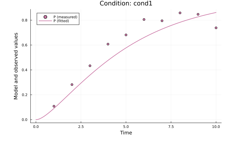
The fitted solution for observable P in the first simulation condition (cond1) can be plotted as:
using Plots
plot(
    res, petab_prob; observable_ids = ["obs_p"],
    condition = :cond1, linewidth = 2.0
)
To plot both observables for the second simulation condition (cond2):
plot(
    res, petab_prob; observable_ids = ["obs_e", "obs_p"],
    condition = :cond2, linewidth = 2.0
)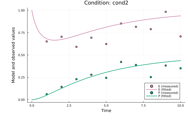
Here, observable_ids is optional since plotting all observables is the default. By default, the observable formula is used in the legend. If formulas are long, the plot can become cluttered and setting obsid_label = true enables labeling by observable ID instead:
plot(
    res, petab_prob; observable_ids = ["obs_e", "obs_p"],
    condition = :cond2, linewidth = 2.0, obsid_label = true
)
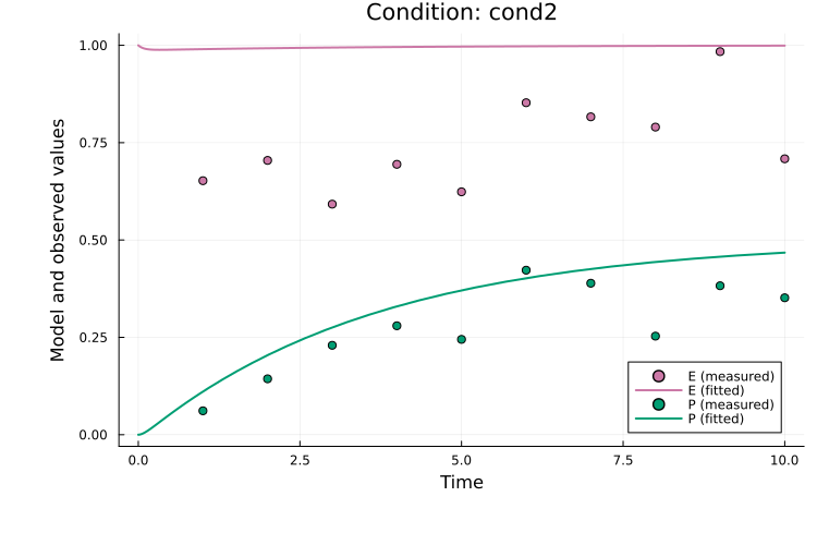
When an estimation result (res) is provided, the fit for the best-found parameter vector is plotted. The fit for any parameter vector in the order expected by the PEtabODEProblem (see get_x) can also be plotted. For example the start guess of the first run (which naturally produces a bad fit):
x0 = res.runs[1].x0
plot(
    x0, petab_prob; observable_ids = ["obs_e", "obs_p"],
    condition = :cond2, linewidth = 2.0
)
To generate plots for all combinations of observables and simulation conditions, use:
comp_dict = get_obs_comparison_plots(res, petab_prob; linewidth = 2.0)comp_dict is a dictionary keyed by condition ID; each value is a dictionary keyed by observable ID. For example, to retrieve the plot for E in cond1:
comp_dict["cond1"]["obs_e"]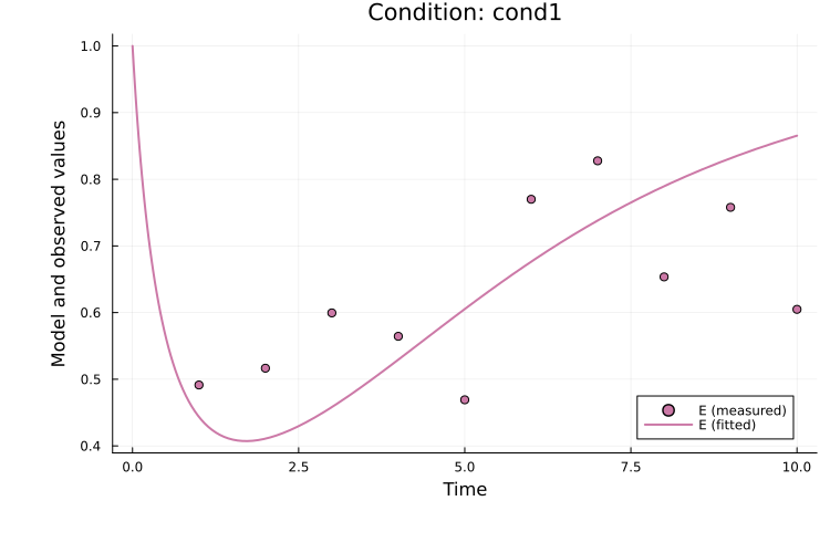
Pre-equilibration
For models with pre-equilibration, specify the condition as pre_eq_id => simulation_id.
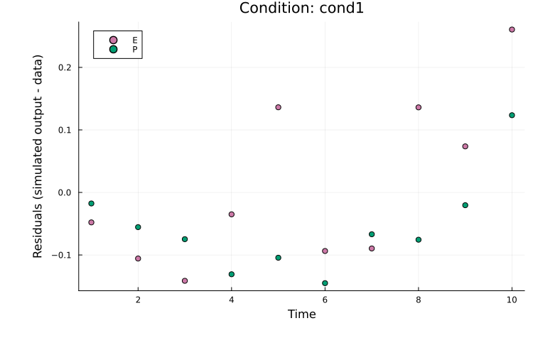
Residuals
Residuals can be plotted in the same way as model-fit plots by setting plot_type = :residuals. For example, to plot residuals for both observables in cond1:
plot(
    res, petab_prob; plot_type = :residuals,
    condition = :cond1, linewidth = 2.0
)
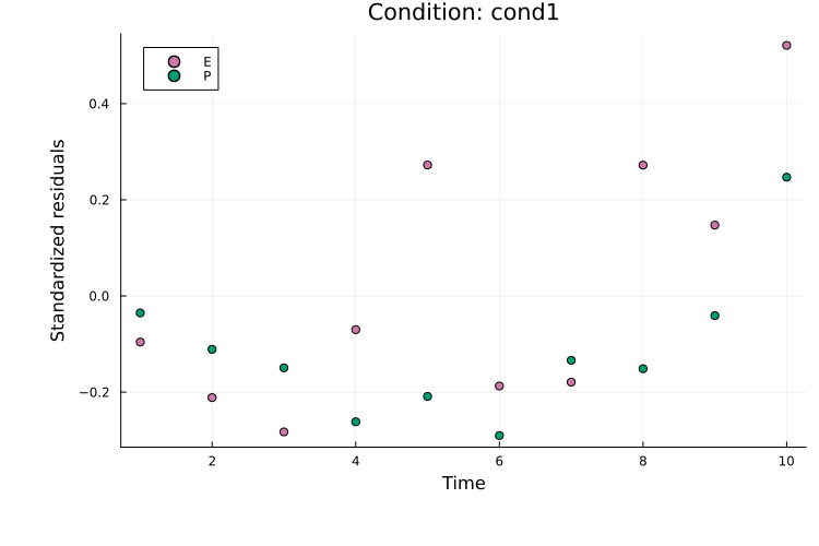
Standardized residuals (normalized by the measurement noise) can be plotted with plot_type = :standardized_residuals:
plot(
    res, petab_prob; plot_type = :standardized_residuals,
    condition = :cond1, linewidth = 2.0
)
References
- A. Raue, M. Schilling, J. Bachmann, A. Matteson, M. Schelke, D. Kaschek, S. Hug, C. Kreutz, B. D. Harms, F. J. Theis and others. Lessons learned from quantitative dynamical modeling in systems biology. PloS one 8, e74335 (2013).