Pre-simulation ML models
Sometimes informative non-time-series data (e.g. images, omics data, ...) are available. One approach to include such data is to use an ML model that takes it as input and, before ODE simulation, maps it to ODE parameters and/or initial conditions.
This tutorial shows how to define SciML problems where an ML model is evaluated pre-simulation to set model parameters and/or initial conditions. It assumes familiarity with the SciML starter tutorial. As a running example, the Michaelis–Menten model from the mechanistic starting tutorial is used:
using Catalyst
sys = @reaction_network begin
    @parameters S0
    @species begin
        S(t) = S0
        E(t) = 50.0
        SE(t) = 0.1
        P(t) = 0.1
    end
    @observables begin
        obs1 ~ S + E
        obs2 ~ P
    end
    c1, S + E --> SE
    c2, SE --> S + E
    c3, SE --> P + E
end
Defining a pre-simulation ML model
A pre-simulation ML model sets one or more ODE parameters and/or initial conditions before each simulation. This is done by (1) defining a Lux.jl model and (2) wrapping it as an MLModel, where inputs and outputs are specified. For example, assume the model parameter c3 is assigned by a simple feed-forward network with input [1.0, 1.0]. The first step is to define the Lux model:
using Lux
lux_model = Lux.Chain(
    Dense(2 => 5, Lux.swish),
    Dense(5 => 1),
)
Then declare the corresponding MLModel, and specify its inputs and outputs:
using PEtab
ml_model = MLModel(
    :net1, lux_model, true; inputs = [1.0, 1.0], outputs = [:c3]
)
MLModel net1
mode: pre-initialization
parameters: 21
inputs: 2-element Vector{Float64}
outputs: [c3]
hint: see model structure in `ml_model.lux_model`Here, true indicates that the ML model is evaluated pre-simulation and assigns the value of c3. To set an initial condition, provide a state ID in outputs. More complex inputs are also possible, such as arrays, parameters from the parameter table, and simulation-condition-specific values (described below).
With the MLModel defined, the remaining PEtab setup is the same as for mechanistic models. Since :c3 is assigned by the ML model, it should not be specified elsewhere:
using DataFrames
@parameters sigma
observables = [
    PEtabObservable(:obs_p, :obs1, 3.0),
    PEtabObservable(:obs_sum, :obs2, sigma),
]

pest = [
    PEtabParameter(:c1),
    PEtabParameter(:c2),
    PEtabParameter(:S0; value = 100.0),
    PEtabParameter(:sigma),
    PEtabMLParameter(:net1), # ML parameters
]

measurements = DataFrame(
    obs_id = ["obs_p", "obs_sum", "obs_p", "obs_sum"],
    time = [1.0, 10.0, 1.0, 20.0],
    measurement = [0.7, 0.1, 1.0, 1.5],
)
Given this, the PEtabModel and associated PEtabODEProblem are created as usual:
petab_model = PEtabModel(
    sys, observables, measurements, pest; ml_models = ml_model
)
petab_prob = PEtabODEProblem(petab_model)
describe(petab_prob)
PEtabODEProblem ReactionSystemModel
Problem statistics
Parameters to estimate: 25
ODE: 4 states, 4 parameters
Observables: 2
Simulation conditions: 1
ML models
net1: (mode=pre-initialization, parameters=21)
Configuration
Gradient method: ForwardDiff
Hessian method: ForwardDiff
ODE solver (nllh): Rodas5P (abstol=1.0e-08, reltol=1.0e-08, maxiters=1e+04)
ODE solver (grad): Rodas5P (abstol=1.0e-08, reltol=1.0e-08, maxiters=1e+04)As seen from the problem statistics, the PEtabODEProblem problem includes both mechanistic parameters and a ML model evaluated pre-simulation.
ml_models must be provided to PEtabModel
Any pre-simulation ML model must also be passed via the ml_models keyword to PEtabModel. For symbolically defined UDEs (as in the SciML starter tutorial), this is not required since PEtab.jl can infer the ML model structure from the model system.
ML input data
The example above uses a simple MLModel input. PEtab.jl supports additional inputs such as condition-specific inputs, high-dimensional arrays (e.g. images), as well as ML models with multiple input arguments in the forward pass. The sections below illustrate these cases and assume familiarity with Simulation conditions. The Michaelis–Menten model from above is used as a working example.
Simulation condition specific (scalar) input
To use condition-specific inputs, entries in MLModel.inputs should be variables that are set using PEtabCondition. For example, assume the inputs are two condition-specific variables input1 and input2. First, define the MLModel:
lux_model = Lux.Chain(
    Dense(2 => 5, Lux.softplus),
    Dense(5 => 1),
)
ml_model = MLModel(
    :net1, lux_model, true; inputs = [:input1, :input2], outputs = [:c3]
)
The values of input1 and input2 are then provided via PEtabCondition. For instance, assign values for two simulation conditions cond1 and cond2:
simulation_conditions = [
    PEtabCondition(:cond1, :input1 => 1.0, :input2 => 3.0),
    PEtabCondition(:cond2, :input1 => 2.0, :input2 => 4.0),
]
The PEtabODEProblem is then created as usual:
# Condition-specific measurements
measurements = DataFrame(
    simulation_id = ["cond1", "cond1", "cond2", "cond2"],
    obs_id        = ["obs_p", "obs_sum", "obs_p", "obs_sum"],
    time          = [5.0, 10.0, 1.0, 10.0],
    measurement   = [0.7, 0.1, 1.0, 1.5],
)

petab_model = PEtabModel(
    sys, observables, measurements, pest; ml_models = ml_model,
    simulation_conditions = simulation_conditions,
)
petab_prob = PEtabODEProblem(petab_model)
As seen, due to the condition specific input the simulated model trajectories differ between conditions:
using Plots
x = get_x(petab_prob)
sol_cond1 = get_odesol(x, petab_prob; condition = :cond1)
sol_cond2 = get_odesol(x, petab_prob; condition = :cond2)
p1 = plot(sol_cond1, title = "cond1")
p2 = plot(sol_cond2, title = "cond2")
plot(p1, p2)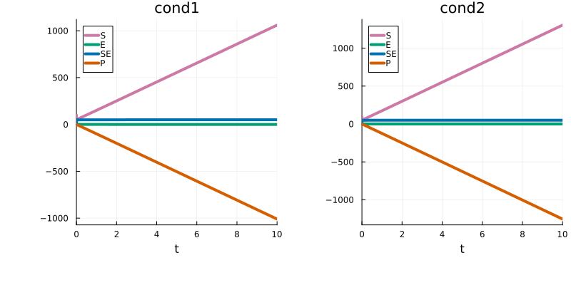
High-dimensional array input
High-dimensional simulation-condition-specific array data (e.g. images) can be mapped to model parameters by assigning an entire MLModel input argument to a PEtab variable, which is then assigned array data in PEtabCondition. For example, let the ML model be a small convolutional network whose input is the condition-specific variable input1:
lux_model = Lux.Chain(
    Conv((5, 5), 3 => 1; cross_correlation = true),
    FlattenLayer(),
    Dense(36 => 1, Lux.softplus),
)
ml_model = MLModel(:net1, lux_model, true; inputs = [:input1], outputs = [:c3])
The value of input1 is then assigned image-like array data in PEtabCondition (random data are used here for illustration):
using StableRNGs
rng = StableRNG(1) # for reproducibility
input_data1 = rand(rng, 10, 10, 3, 1)
input_data2 = rand(rng, 10, 10, 3, 1)
simulation_conditions = [
    PEtabCondition(:cond1, :input1 => input_data1),
    PEtabCondition(:cond2, :input1 => input_data2),
]
2-element Vector{PEtabCondition}:
PEtabCondition cond1: input1 => 10×10×3×1 Array{Float64, 4}
PEtabCondition cond2: input1 => 10×10×3×1 Array{Float64, 4}The input shape must match what lux_model expects. Given this, the PEtabODEProblem is created as usual, and as seen simulated model trajectories differ between conditions:
petab_model = PEtabModel(
    sys, observables, measurements, pest; ml_models = ml_model,
    simulation_conditions = simulation_conditions,
)
petab_prob = PEtabODEProblem(petab_model)

x = get_x(petab_prob)
sol_cond1 = get_odesol(x, petab_prob; condition = :cond1)
sol_cond2 = get_odesol(x, petab_prob; condition = :cond2)
p1 = plot(sol_cond1, title = "cond1")
p2 = plot(sol_cond2, title = "cond2")
plot(p1, p2)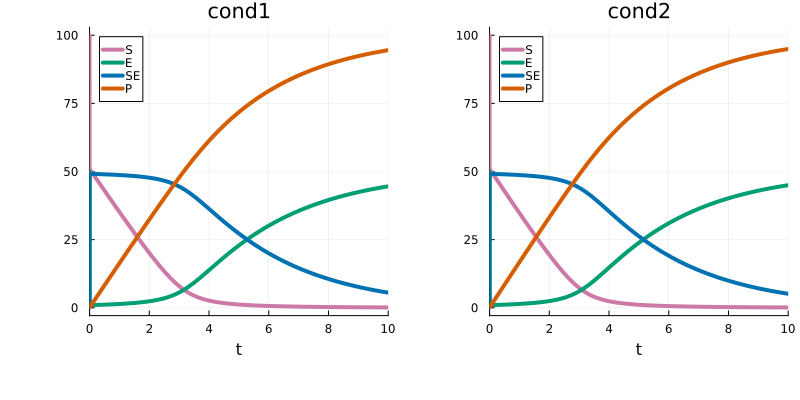
Multiple input arguments
The forward pass of an ML model can take multiple input arguments (e.g. a feature vector and a covariate). This is handled by providing inputs as a tuple, with one entry per input argument. For example, let the first input argument be [1.0, 2.0] and the second be the condition-specific variable input2:
using Lux
lux_model = @compact(
    layer1 = Dense(3 => 5, Lux.swish),
    layer2 = Dense(5 => 1),
) do (x1, x2)
    x = cat(x1, x2; dims = 1)
    h = layer1(x)
    out = layer2(h)
    @return out
end

ml_model = MLModel(
    :net1, lux_model, true; inputs = ([1.0, 2.0], [:input2]), outputs = [:c3]
)
With input2 assigned in PEtabCondition, the PEtabODEProblem can be created as usual:
simulation_conditions = [
    PEtabCondition(:cond1, :input2 => 1.0),
    PEtabCondition(:cond2, :input2 => 2.0),
]

petab_model = PEtabModel(
    sys, observables, measurements, pest; ml_models = ml_model,
    simulation_conditions = simulation_conditions,
)
petab_prob = PEtabODEProblem(petab_model)
PEtabODEProblem ReactionSystemModel: 30 parameters to estimate
(for more statistics, call `describe(petab_prob)`)Performance tips
When the ML model is evaluated pre-simulation, gradient computations can often be sped up by setting split_over_conditions = true (the default) when building the PEtabODEProblem. More details are provided in Speeding up pre-simulation SciML problems.