SciML starter tutorial: Universal Differential Equations (UDEs)
Hybrid scientific machine learning (SciML) combines mechanistic (ODE) models with machine learning (ML) models [22]. PEtab.jl supports three SciML problem types, and any combination of them:
ML model inside the ODE dynamics. This covers both Universal Differential Equations (UDEs), also called grey-box and hybrid neural ODEs [23, 24], as well as neural ODEs (NODEs) [25].
ML model in the observable formula which links ODE output to measurement data.
Pre-simulation ML model, where the ML model is evaluated before simulation to map input data (e.g. high-dimensional images) to ODE parameters and/or initial conditions.
This tutorial introduces SciML functionality in PEtab.jl using the UDE case. Other tutorials in this section cover the remaining cases. Familiarity with setting up a PEtab problem for mechanistic models is assumed; see the PEtab.jl starting tutorial.
While this tutorial focuses on a simple use-case, note that SciML support is implemented on top of the functionality for mechanistic models. Thus, features for mechanistic models (e.g. simulation conditions and events) are also supported for SciML problems.
Input problem
As a running example, we use the following two-state ODE model:
with initial conditions
To turn this into a UDE [22], we assume the production term for
Where
To estimate model parameters, measurements of both d and the parameters of NN.
Creating a PEtab SciML problem
A PEtab SciML parameter estimation problem (i.e., PEtabODEProblem) is created largely the same way as for a mechanistic model. The difference is that one or more Lux.jl neural networks are defined and embedded into the problem.
Defining the ML model
PEtab.jl only supports Lux.jl ML models. To be compatible, the Lux model must define a set of layers with unique identifiers together with a forward pass. This is most easily done using Lux.Chain:
using Lux
lux_model = Lux.Chain(
    Lux.Dense(1 => 3, Lux.softplus, use_bias = false),
    Lux.Dense(3 => 3, Lux.softplus, use_bias = false),
    Lux.Dense(3 => 1, Lux.softplus, use_bias = false),
)
Chain(
layer_1 = Dense(1 => 3, softplus, use_bias=false), # 3 parameters
layer_2 = Dense(3 => 3, softplus, use_bias=false), # 9 parameters
layer_3 = Dense(3 => 1, softplus, use_bias=false), # 3 parameters
) # Total: 15 parameters,
# plus 0 states.Here, softplus activation function is used to keep the output positive.
Defining the dynamic UDE model
An UDE dynamic model is most easily created using ModelingToolkitNeuralNets. The first step is to create a symbolic neural network from the Lux model:
using ModelingToolkitNeuralNets
@SymbolicNeuralNetwork NN, theta = lux_model
Here theta is the network parameter vector, and NN is the neural network which can be embedded into a ModelingToolkit model:
using ModelingToolkitBase
using ModelingToolkitBase: t_nounits as t, D_nounits as D

@parameters d
@variables X(t)=2.0 Y(t)=0.1
eqs = [
    D(X) ~ NN([Y], theta)[1] - d * X
    D(Y) ~ X - d * Y
]
@mtkcompile sys_ude = System(eqs, t)
Alternatively, the UDE can be formulated as a Catalyst ReactionSystem:
using Catalyst

# Scalar NN rate depending on Y.
A(z) = NN([z], theta)
rn_ude = @reaction_network begin
    @species begin
        X(t) = 2.0
        Y(t) = 0.1
    end
    @parameters d
    # Reactions
    $A(Y)[1], 0 --> X
    d, X --> 0
    1.0, X --> X + Y
    d, Y --> 0
end
When embedding a neural network into a ReactionSystem, it must be introduced via a symbolic function (here A(z)) and can only be used in the parameter position of a reaction.
For more on symbolic UDE creation, see the ModelingToolkitNeuralNets documentation.
Defining ML parameters to estimate
For each ML-model, a PEtabMLParameter must be declared to specify whether its parameters are estimated. Thereby, when specifying the parameters-to-estimate vector for a SciML problem, both mechanistic parameters (PEtabParameter) and ML parameters (PEtabMLParameter) must be included in the parameter vector:
using PEtab
pest = [
    PEtabMLParameter(:theta),
    PEtabParameter(:d; scale = :log10)
]
2-element Vector{Any}:
PEtabMLParameter theta: estimate
PEtabParameter d: estimate (scale = log10, bounds = [1.0e-03, 1.0e+03])A PEtabMLParameter can optionally be given an initial value, priors, and be fixed to specific value. Note, parameter d is estimated on log10 scale to enforce positivity.
Measurements and observables
Measurements and observables are defined as for a mechanistic PEtabODEProblem. For the running example, we use simulated data:
# Simulate data
using DataFrames, OrdinaryDiffEqTsit5, StableRNGs
rng = StableRNGs.StableRNG(3)
@variables X(t) Y(t)
@parameters v K n d
eqs_true = [D(X) ~ v * (Y^n) / (K^n + Y^n) - d*X
D(Y) ~ X - d*Y]
@mtkcompile sys_true = System(eqs_true, t)
u0 = [X => 2.0, Y => 0.1]
ps_true = [v => 1.1, K => 2.0, n => 3.0, d => 0.5]
tend = 66.0
ode_true = ODEProblem(sys_true, [u0; ps_true], (0.0, tend))
sol = solve(
ode_true, Tsit5(); abstol = 1e-8, reltol = 1e-8, saveat = 0:2:tend
)
data_X = sol[1, :] .+ randn(rng, length(sol.t)) .* 0.5
data_Y = sol[2, :] .+ randn(rng, length(sol.t)) .* 0.7
df1 = DataFrame(obs_id = "obs_X", time = sol.t, measurement = data_X)
df2 = DataFrame(obs_id = "obs_Y", time = sol.t, measurement = data_Y)
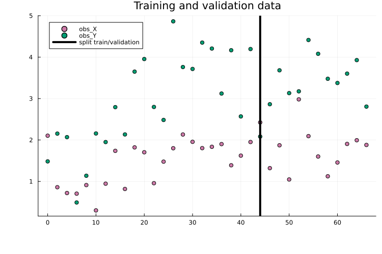
measurements = vcat(df1, df2)For SciML models, it is often useful to set aside validation data to monitor overfitting. Here, the first 2/3 of time points are used for training and the remaining 1/3 for validation:
using Plots
measurements_train = filter(row -> row.time <= 44.0, measurements)
measurements_val = filter(row -> row.time > 44.0, measurements)
scatter(
    measurements.time, measurements.measurement, group = measurements.obs_id,
    title = "Training and validation data"
)
vline!(
    [44.0], label = "split train/validation", color = "black"
)
Lastly, since both X and Y are assumed measured, the observables are:
observables = [
    PEtabObservable(:obs_X, :X, 0.5),
    PEtabObservable(:obs_Y, :Y, 0.7),
]
2-element Vector{PEtabObservable}:
PEtabObservable obs_X: data ~ Normal(μ=X, σ=0.5)
PEtabObservable obs_Y: data ~ Normal(μ=Y, σ=0.7)Bringing it all together
Given the dynamic model (sys_ude or rn_ude), measurements, observables, and parameters to estimate, a PEtabODEProblem is created the same way as for a mechanistic problem. When using training/validation (and optionally test) splits, a separate problem should be created for each split. For example, for the training data the first step is to create a PEtabModel:
# Via ReactionSystem
model_ude_train = PEtabModel(rn_ude, observables, measurements_train, pest)
# Via ODESystem
model_ude_train = PEtabModel(sys_ude, observables, measurements_train, pest)
Given a PEtabModel, a PEtabODEProblem can then be constructed:
petab_prob_train = PEtabODEProblem(model_ude_train)
describe(petab_prob_train)
PEtabODEProblem ODESystemModel
Problem statistics
Parameters to estimate: 16
ODE: 2 states, 16 parameters
Observables: 2
Simulation conditions: 1
ML models
theta: (mode=simulation, parameters=15)
Configuration
Gradient method: ForwardDiff
Hessian method: ForwardDiff
ODE solver (nllh): Tsit5 (abstol=1.0e-08, reltol=1.0e-08, maxiters=1e+04)
ODE solver (grad): Tsit5 (abstol=1.0e-08, reltol=1.0e-08, maxiters=1e+04)As seen from the problem summary, the problem includes both mechanistic and ML parameters to estimate. It is further seen the non-stiff ODE solver Tsit5() is used and gradients are computed with ForwardDiff. These options can be changed, and the same PEtabODEProblem options are supported as for mechanistic models.
To compute validation loss (and run other analyses such as plotting), create a PEtabODEProblem using the validation measurements:
# Via ReactionSystem
model_ude_val = PEtabModel(rn_ude, observables, measurements_val, pest)
petab_prob_val = PEtabODEProblem(model_ude_val)
Parameter estimation (model training)
SciML problems can be trained using the same approaches as mechanistic models (e.g. multi-start local optimization with a BFGS-based method via calibrate). In practice, SciML training often benefits from optimizers commonly used for ML [15], such as the Adam optimizer [14]. Adam, and other common ML optimizers are available in Optimisers.jl.
Like most optimizers, Adam requires a start guess which can be generated with:
using StableRNGs
rng = StableRNGs.StableRNG(42) # for reproducibility
x0 = get_startguesses(rng, petab_prob_train, 1)
ComponentVector{Float64}(log10_d = 0.48308917611117286, theta = (layer_1 = (weight = [-0.038298919796943665; 0.8650590777397156; 0.7111778855323792;;]), layer_2 = (weight = [0.9691276550292969 0.11354947090148926 -0.64198899269104; -0.9428482055664062 0.9947323799133301 0.7659111022949219; 0.8692448139190674 0.7045483589172363 0.3672807216644287]), layer_3 = (weight = [0.9935319423675537 -0.6066112518310547 -0.90108323097229])))The start guess includes both mechanistic parameters (e.g. x0.d) and ML parameters (e.g. x0.theta). By default, get_startguesses initializes ML parameters using the initializers in the Lux model. While not needed here, training often improves by initializing ML parameters to smaller values [26].
With a start guess available, calibrate can train with any optimizer from Optimisers.jl. For example, to train for 7500 epochs/iterations with Adam:
using Optimisers
learning_rate = 1e-3
res = calibrate(
    petab_prob_train, x0, Optimisers.Adam(learning_rate);
    options = OptimisersOptions(iterations = 7500),
)
PEtabOptimisationResult
min(f) = 3.88e+01
Parameters estimated = 16
Optimiser iterations = 7500
Runtime = 7.6e+01s
Optimiser algorithm = Optimisers.AdamBoth calibrate and calibrate_multistart run the provided update rule for the number of iterations specified in OptimisersOptions. For more fine-grained control (e.g. learning rate schedules and early stopping), a custom training loop must be implemented.
A custom loop can be written leveraging that the objective and its gradient can be computed with petab_prob_train.nllh(x) and petab_prob_train.grad(x), respectively. For example, to train for 7500 epochs/iterations with Adam:
using Optimisers
n_epochs = 7500
x = deepcopy(x0)
learning_rate = 1e-3

state = Optimisers.setup(Optimisers.Adam(learning_rate), x)
for epoch in 1:n_epochs
    g = petab_prob_train.grad(x)
    state, x = Optimisers.update(state, x, g)

    # Stop if the objective cannot be evaluated (e.g. simulation failure)
    if !isfinite(petab_prob_train.nllh(x))
        break
    end
end
By plotting the fitted model, we see that it fits the training data well:
plot(x, petab_prob_train, title = "Training data fit")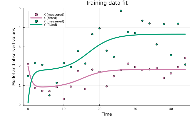
Plotting the validation fit also shows that the fitted model generalizes well:
plot(x, petab_prob_val, title = "Validation data fit")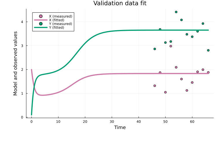
As one of many possible downstream analyses, we can compare the learned neural network to the true function it aims to approximate. The learned function can be plotted using PEtab's plotting interface with the :best_function and :function_ensemble options:
plot(x, petab_prob_train; plot_type = :best_function, label = "Fitted function", linestyle = :dash, lw = 5)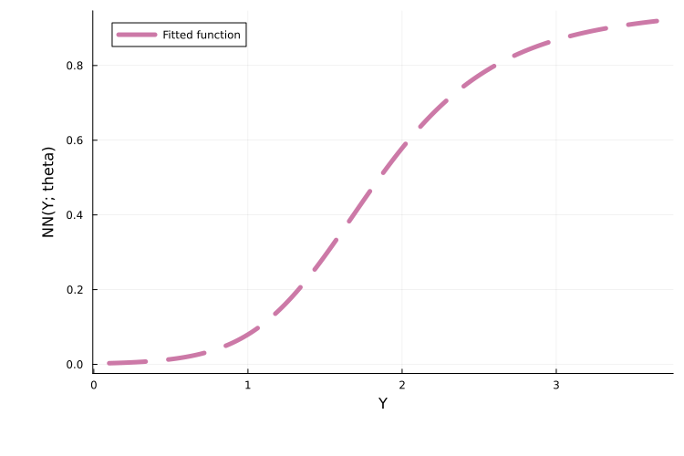
We can then overlay the true function to assess the approximation quality:
true_func(y) = 1.1 * (y^3) / (2^3 + y^3)
plot!(true_func, 0.0, 3.5; label = "True function", lw = 3)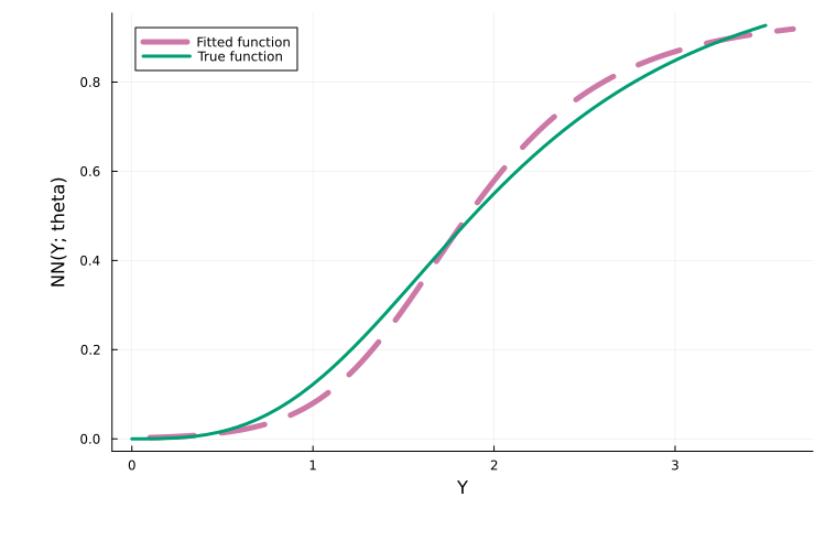
In this example, the learned function closely matches the true function. For a full overview of plotting options for learned functions, see here.
The above training loop above is intentionally minimal. In practice, Optimisers.jl and related packages can be used to add learning-rate schedules, gradient clipping, early stopping, and logging. It is also worth noting that plain Adam is often inefficient for SciML problems, and to address this PEtab.jl supports more effective strategies such as curriculum training, multiple shooting, and combinations thereof (see below).
Next steps
This tutorial showed how to define a PEtabODEProblem for a SciML problem. For all available options when building SciML problems (e.g. PEtabMLParameter settings), see the API documentation. For additional features, including SciML problem types beyond UDEs, see the following tutorials:
Extended UDE tutorial: Define the UDE model as an
ODEProblemfor more control over the problem setup.ML models in observables: define an ML model in the observable formula of a
PEtabObservable(e.g. to correct model misspecification).Pre-simulation ML models: define ML models that map input data (e.g. high-dimensional images) to ODE parameters or initial conditions prior to model simulation.
Importing PEtab SciML: import problems in the PEtab-SciML standard format.
Plotting learned functions: How to plot the learned neural network function for UDE problems.
In addition, this tutorial showed how to train a UDE via a simple Adam training loop. More efficient training strategies are supported via PEtabTraining.jl (e.g. curriculum learning and multiple shooting); see SciML training strategies.
Lastly, as for mechanistic models, PEtabODEProblem has many configurable options for SciML problems. A discussion of defaults and recommendations is available in Default PEtabODEProblem options.
Copy pasteable example
using Catalyst, ComponentArrays, Lux, ModelingToolkitBase,
    ModelingToolkitNeuralNets, PEtab
using ModelingToolkitBase: t_nounits as t, D_nounits as D

# MLModel
lux_model = Lux.Chain(
    Lux.Dense(1 => 3, Lux.softplus, use_bias = false),
    Lux.Dense(3 => 3, Lux.softplus, use_bias = false),
    Lux.Dense(3 => 1, Lux.softplus, use_bias = false),
)

# UDE-system
@SymbolicNeuralNetwork NN, theta = lux_model
@parameters d
@variables X(t)=2.0 Y(t)=0.1
eqs = [
    # Equations
    D(X) ~ NN([Y], theta)[1] - d * X
    D(Y) ~ X - d * Y
]
@mtkcompile sys_ude = System(eqs, t)

# UDE-system via ReactionSystem
using Catalyst

# Scalar NN rate depending on Y.
A(z) = NN([z], theta)
rn_ude = @reaction_network begin
    @species begin
        X(t) = 2.0
        Y(t) = 0.1
    end
    @parameters d

    $A(Y)[1], 0 --> X
    d, X --> 0
    1.0, X --> X + Y
    d, Y --> 0
end

# Parameters to estimate
pest = [
    PEtabMLParameter(:theta),
    PEtabParameter(:d; scale = :log10)
]

# Observables linking model output to data
observables = [
    PEtabObservable(:obs_X, :X, 0.5),
    PEtabObservable(:obs_Y, :Y, 0.7),
]

# Simulate data
using DataFrames, OrdinaryDiffEqTsit5, StableRNGs
rng = StableRNGs.StableRNG(3)

@variables X(t) Y(t)
@parameters v K n d
eqs_true = [D(X) ~ v * (Y^n) / (K^n + Y^n) - d*X
       D(Y) ~ X - d*Y]
@mtkcompile sys_true = System(eqs_true, t)
u0 = [X => 2.0, Y => 0.1]
ps_true = [v => 1.1, K => 2.0, n => 3.0, d => 0.5]

tend = 66.0
ode_true = ODEProblem(sys_true, [u0; ps_true], (0.0, tend))
sol = solve(
    ode_true, Tsit5(); abstol = 1e-8, reltol = 1e-8, saveat = 0:2:tend
)
data_X = sol[1, :] .+ randn(rng, length(sol.t)) .* 0.5
data_Y = sol[2, :] .+ randn(rng, length(sol.t)) .* 0.7
df1 = DataFrame(obs_id = "obs_X", time = sol.t, measurement = data_X)
df2 = DataFrame(obs_id = "obs_Y", time = sol.t, measurement = data_Y)
measurements = vcat(df1, df2)

# Split data into training and validation sets
using Plots
measurements_train = filter(row -> row.time <= 44.0, measurements)
measurements_val = filter(row -> row.time > 44.0, measurements)
scatter(
    measurements.time, measurements.measurement,  group = measurements.obs_id,
    label = "Training and validation data"
)
vline!(
    [44.0], label = "split train/validation", color = "black"
)

# Create parameter estimation problem
model_ude_train = PEtabModel(
    sys_ude, observables, measurements_train, pest
)
petab_prob_train = PEtabODEProblem(model_ude_train)

# Create corresponding problem to compute validation loss
model_ude_val = PEtabModel(
    sys_ude, observables, measurements_val, pest
)
petab_prob_val = PEtabODEProblem(model_ude_val)

# Get random start-guess for model training
rng = StableRNG(42) # for reproducibility
x0 = get_startguesses(rng, petab_prob_train, 1)

# Use built PEtab calibrate to train
using Optimisers
learning_rate = 1e-3
res = calibrate(
    petab_prob_train, x0, Optimisers.Adam(learning_rate);
    options = OptimisersOptions(iterations = 7500),
)

# Custom written Adam training loop
n_epochs = 7500
x = deepcopy(x0)
learning_rate = 1e-3
state = Optimisers.setup(Adam(learning_rate), x)
for epoch in 1:n_epochs
    g = petab_prob_train.grad(x)
    state, x = Optimisers.update(state, x, g)

    # Stop if the objective cannot be evaluated (e.g. simulation failure)
    if !isfinite(petab_prob_train.nllh(x))
        break
    end
end
plot(x, petab_prob_train, title = "Training data fit")

# Plot validation fit
plot(x, petab_prob_val, title = "Validation data fit")

# Plot fitted function.
plot(
    res, petab_prob_train; plot_type = :best_function,
    label = "Fitted function", linestyle = :dash, lw = 5
)
# Overlays the fitted function with the true function.
true_func(y) = 1.1 * (y^3) / (2^3 + y^3)
plot!(true_func, 0.0, 3.5; label = "True function", lw = 3)
References
D. P. Kingma and J. Ba. Adam: A method for stochastic optimization, arXiv preprint arXiv:1412.6980 (2014).
M. Philipps, N. Schmid and J. Hasenauer. Current state and open problems in universal differential equations for systems biology, npj Systems Biology and Applications 11, 101 (2025).
C. Rackauckas, Y. Ma, J. Martensen, C. Warner, K. Zubov, R. Supekar, D. Skinner, A. Ramadhan and A. Edelman. Universal differential equations for scientific machine learning, arXiv preprint arXiv:2001.04385 (2020).
J. Brucker, R. Behmann, W. G. Bessler and R. Gasper. Neural ordinary differential equations for grey-box modelling of lithium-ion batteries on the basis of an equivalent circuit model. Energies 15, 2661 (2022).
B. J. Zou, M. E. Levine, D. P. Zaharieva, R. Johari and E. B. Fox. Hybrid2 neural ODE causal modeling and an application to glycemic response. In: Proceedings of the 41st International Conference on Machine Learning, Vol. 235 of ICML'24 (JMLR.org, Vienna, Austria, Jul 2024); pp. 62934–62963. Accessed on Apr 20, 2026.
R. T. Chen, Y. Rubanova, J. Bettencourt and D. K. Duvenaud. Neural ordinary differential equations. Advances in neural information processing systems 31 (2018).
P. Kidger. On neural differential equations, arXiv preprint arXiv:2202.02435 (2022).